Power of abess Library: Empirical Comparison

Introduction

In this part, we are going to explore the power of the abess package using simulated data. We compare the abess package with popular Python packages: scikit-learn for linear and logistic regressions in the following section. (Actually, we also compare with python-glmnet, statsmodels and L0bnb, but the python-glmnet presents a poor prediction error, the statsmodels runs slow and the L0bnb cannot adaptively choose sparsity level. So their results are not showed here.)

Simulation Setting

Both packages are compared in three aspects including the prediction performance, the variable selection performance, and the computation efficiency.

• The prediction performance of the linear model is measured by \(||y−\hat{y}||_2\) on a test set and for logistic regression this is measured by the area under the ROC curve (AUC).

• The coefficient estimation performance are measured by the coefficient error \(||\beta - \hat{\beta}||_2\).

• For the variable selection performance, we compute true positive rate (TPR, which is the proportion of variables in the active set that are correctly identified) and the false positive rate (FPR, which is the proportion of the variables in the inactive set that are falsely identified as a signal).

• Timings of the CPU execution are recorded in seconds, and all of methods select the best model among 100 models under different regularization strength or support size.

The simulated data are made by abess.datasets.make_glm_data(). The number of predictors is \(p=8000\) and the size of data is \(n=500\). The true coefficient contains \(k=10\) nonzero entries uniformly distributed in \([b,B]\):

• For linear regression (family = "gaussian"), we set \(b = 5\sqrt{2\ln p / n}\) and \(B = 100b\).

• For logistic regression (family = "binomial"), we set \(b = 10\sqrt{2\ln p / n}\) and \(B = 5b\).

In each regression, we test for both low (\(\rho=0.1\)) and high correlation (\(\rho=0.7\)) scenarios. What’s more, a random noise generated from a standard Gaussian distribution is added to the linear predictor \(x^{\top} \beta\) for linear regression.

All the performances are averaged over 20 replications. All experiments are evaluated on a Arch Linux platform with Intel(R) Core(TM) i5-6500 CPU @ 3.20GHz and 16 RAM.

$ python abess/docs/simulation/Python/plot_results_figure.py

Numerical Results

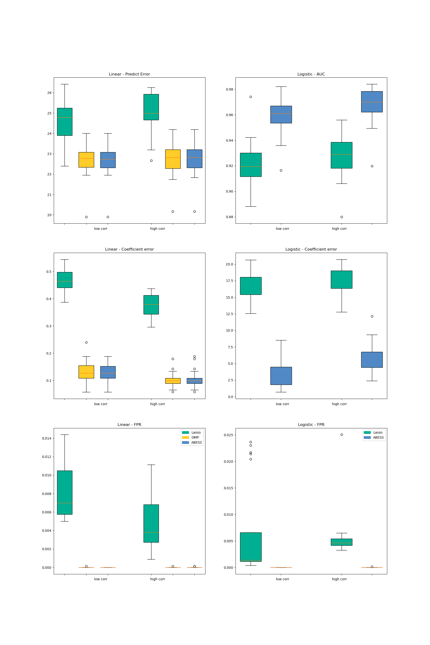
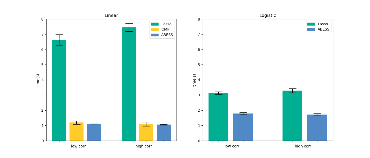
For linear regression, we compare three methods in the two packages: Lasso, OMP and abess. For logistic regression, we compare two methods: lasso and abess. The results are presented in the following pictures. The first column is the result of linear regression and the second one is of logistic regression.

• Firstly, among all of the methods implemented in different packages, the estimator obtained by the abess package shows both the best prediction performance and the best coefficient error.

• Secondly, the estimator obtained by the abess package can reasonably control FPR in a low level while the TPR stays at 1. (Since all methods’ TPR are 1, the figure is not plotted.)

• Furthermore, our abess package is highly efficient compared with other packages, especially in the linear regression.

For abess R library's performance, please view https://abess-team.github.io/abess/articles/v11-power-of-abess.html.

sphinx_gallery_thumbnail_path = 'Tutorial/figure/timings.png'