Robust Principal Component Analysis

This notebook introduces what is adaptive best subset selection robust principal component analysis (RobustPCA) and then we show how it works using abess package on an artificial example.

PCA

Principal component analysis (PCA) is an important method in the field of data science, which can reduce the dimension of data and simplify our model. It solves an optimization problem like:

\[\max_{v} v^T\Sigma v,\qquad s.t.\quad v^Tv=1.\]

where \(\Sigma = X^TX/(n-1)\) and \(X\in \mathbb{R}^{n\times p}\) is the centered sample matrix with each row containing one observation of \(p\) variables.

Robust-PCA (RPCA)

However, the original PCA is sensitive to outliers, which may be unavoidable in real data:

• Object has extreme performance due to fortuity, but he/she shows normal in repeated tests;

• Wrong observation/recording/computing, e.g. missing or dead pixels, X-ray spikes.

In this situation, PCA may spend too much attention on unnecessary variables. That's why Robust-PCA (RPCA) is presented, which can be used to recover the (low-rank) sample for subsequent processing.

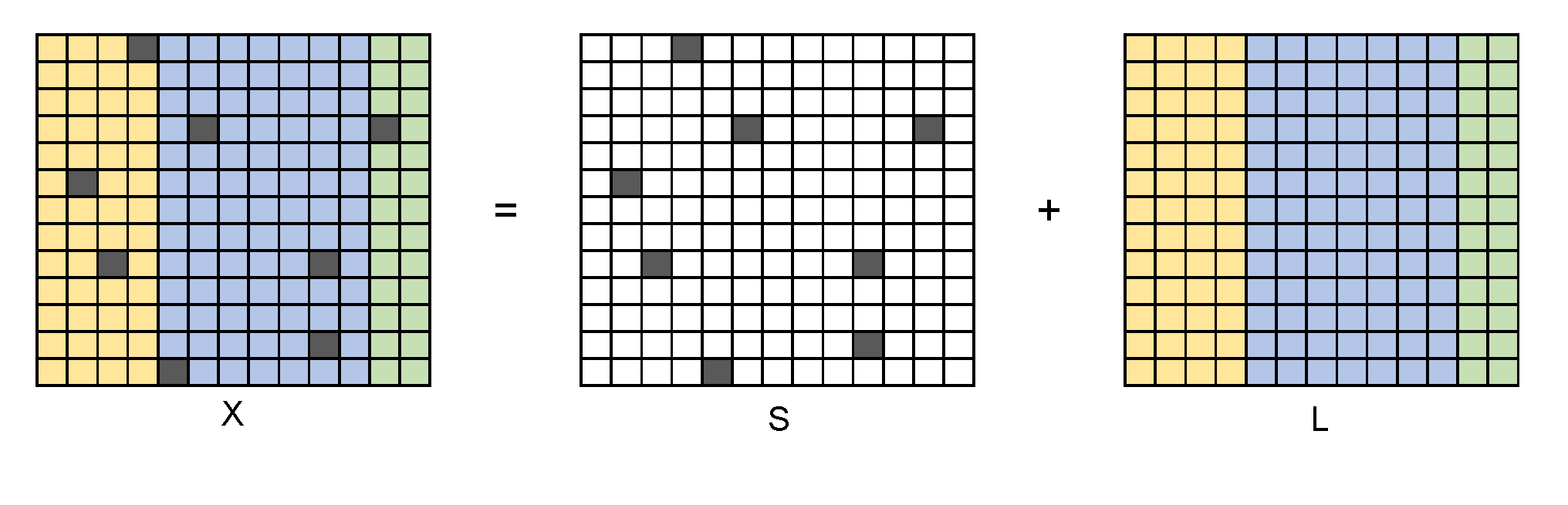
In mathematics, RPCA manages to divide the sample matrix \(X\) into two parts:

\[X = S + L,\]

where \(S\) is the sparse "outlier" matrix and \(L\) is the "information" matrix with a low rank. Generally, we also suppose \(S\) is not low-rank and \(L\) is not sparse, in order to get unique solution.

In Lagrange format,

\[\min _{S, L}\|X-S-L\|_{F} \leq \varepsilon, s . t . \quad \operatorname{rank}(L)=r,\|S\|_{0} \leq s\]

where \(s\) is the sparsity of \(S\). After RPCA, the information matrix \(L\) can be used in further analysis.

Note that it does NOT deal with "noise", which may stay in \(L\) and need further procession.

Hard Impute

To solve its sub-problem, RPCA under known outlier positions, we follow a process called "Hard Impute". The main idea is to estimate the outlier values by precise values with KPCA, where \(K=r\).

Here are the steps:

1. Input \(X, outliers, M, \varepsilon\), where \(outliers\) records the non-zero positions in \(S\);

2. Denote \(X_{\text{new}} \leftarrow {\bf 0}\) with the same shape of \(X\);

3. For \(i = 1,2, \dots, M\):

   • \(X_{\text{old}} = \begin{cases} X_{\text{new}},&\text{for } outliers\\X,&\text{for others}\end{cases}\);

   • Form KPCA on \(X_{\text{old}}\) with \(K=r\), and denote \(v\) as the eigenvectors;

   • \(X_{\text{new}} = X_{\text{old}}\cdot v\cdot v^T\);

   • If \(\|X_{\text{new}} - X_{\text{old}}\| < \varepsilon\), break;

   End for;

4. Return \(X_{\text{new}}\) as \(L\);

where \(M\) is the maximum iteration times and \(\varepsilon\) is the convergence coefficient.

The final \(X_{\text{new}}\) is supposed to be \(L\) under given outlier positions.

RPCA Application

Recently, RPCA is more widely used, for example,

• Video Decomposition: in a surveillance video, the background may be unchanged for a long time while only a few pixels (e.g. people) update. In order to improve the efficiency of storing and analysis, we need to decomposite the video into background and foreground. Since the background is unchanged, it can be stored well in a low-rank matrix, while the foreground, which is usually quite small, can be indicated by a sparse matrix. That is what RPCA does.

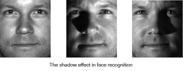
• Face recognition: due to complex lighting conditions, a small part of the facial features may be unrecognized (e.g. shadow). In the face recognition, we need to remove the effects of shadows and focus on the face data. Actually, since the face data is almost unchanged (for one person), and the shadows affect only a small part, it is also a suitable situation to use RPCA. Here are some examples:

Simulated Data Example

Fitting model

Now we generate an example with \(100\) rows and \(100\) columns with \(200\) outliers. We are looking forward to recovering it with a low rank \(10\).

from abess.decomposition import RobustPCA
import numpy as np


def gen_data(n, p, s, r, seed=0):
    np.random.seed(seed)
    outlier = np.random.choice(n * p, s, replace=False)
    outlier = np.vstack((outlier // p, outlier % p)).T
    L = np.dot(np.random.rand(n, r), np.random.rand(r, n))
    S = np.zeros((n, p))
    S[outlier[:, 0], outlier[:, 1]] = float(np.random.randn(1)) * 10
    X = L + S
    return X, S


n = 100     # rows
p = 100     # columns
s = 200     # outliers
r = 10      # rank(L)

X, S = gen_data(n, p, s, r)
print(f'X shape: {X.shape}')
# print(f'outlier: \n{outlier}')

X shape: (100, 100)

In order to use our program, users should call RobustPCA() and give the outlier number to support_size. Note that it can be a specific integer or an integer interval. For the latter case, a support size will be chosen by information criterion (e.g. GIC) adaptively.

# support_size can be a interval like `range(s_min, s_max)`
model = RobustPCA(support_size=s)

It is quite easy to fit this model, with RobustPCA.fit function. Given the original sample matrix \(X\) and \(rank(L)\) we want, the program will give a result quickly.

model.fit(X, r=r)  # r=rank(L)

RobustPCA(support_size=200)

In a Jupyter environment, please rerun this cell to show the HTML representation or trust the notebook.
On GitHub, the HTML representation is unable to render, please try loading this page with nbviewer.org.

Now the estimated outlier matrix is stored in model.coef_.

S_est = model.coef_
print(f'estimated sparsity: {np.count_nonzero(S_est)}')

estimated sparsity: 200

More on the result

To check the performance of the program, we use TPR, FPR as the criterion.

def TPR(pred, real):
    TP = (pred != 0) & (real != 0)
    P = (real != 0)
    return sum(sum(TP)) / sum(sum(P))


def FPR(pred, real):
    FP = (pred != 0) & (real == 0)
    N = (real == 0)
    return sum(sum(FP)) / sum(sum(N))


def test_model(pred, real):
    tpr = TPR(pred, real)
    fpr = FPR(pred, real)
    return np.array([tpr, fpr])


print(f'[TPR  FPR] = {test_model(S_est, S)}')

[TPR  FPR] = [0.925      0.00153061]

We can also change different random seed to test for more situation:

M = 30  # use 30 different seed
res = np.zeros(2)
for seed in range(M):
    X, S = gen_data(n, p, s, r, seed)
    model = RobustPCA(support_size=s).fit(X, r=r)
    res += test_model(model.coef_, S)

print(f'[TPR  FPR] = {res/M}')

[TPR  FPR] = [0.89866667 0.00206803]

Under all of these situations, RobustPCA has a good performance.

R tutorial

For R tutorial, please view https://abess-team.github.io/abess/articles/v08-sPCA.html.

sphinx_gallery_thumbnail_path = 'Tutorial/figure/rpca_shadow.png'