Work with scikit-learn

abess is very easy to work with the famous package scikit-learn, and here is an example. We going to illustrate the integration of the abess with scikit-learn’s pre-processing and model selection modules to build a non-linear model for diagnosing malignant tumors. Let start with importing necessary dependencies:

from abess.linear import LogisticRegression
from sklearn.datasets import load_breast_cancer
from sklearn.pipeline import Pipeline
from sklearn.metrics import roc_auc_score, make_scorer, roc_curve, auc
from sklearn.preprocessing import PolynomialFeatures
from sklearn.model_selection import GridSearchCV

Establish the process

Suppose we would like to extend the original variables to their interactions, and then do LogisticRegression on them. This can be record with Pipeline:

pipe = Pipeline([
    ('poly', PolynomialFeatures(include_bias=False)),   # without intercept
    ('alogistic', LogisticRegression())
])

Parameter grid

We can give different parameters to model and let the program choose the best. Here we should give parameters for PolynomialFeatures, for example:

param_grid = {
    # whether the "self-combination" (e.g. X^2, X^3) exists
    'poly__interaction_only': [True, False],
    'poly__degree': [1, 2, 3]                   # the degree of polynomial
}

Note that the program would try all combinations of what we give, which means that there are \(2\times3=6\) combinations of parameters will be tried.

Criterion

After giving a grid of parameters, we should define what is a "better" result. For example, the AUC (area under ROC curve) can be a criterion and the larger, the better.

scorer = make_scorer(roc_auc_score, greater_is_better=True)

Cross Validation

For more accurate results, cross validation (CV) is often formed. In this example, we use 5-fold CV for parameters searching:

grid_search = GridSearchCV(pipe, param_grid, scoring=scorer, cv=5)

Model fitting

Eveything is prepared now. We can simply load the data and put it into grid_search:

X, y = load_breast_cancer(return_X_y=True)
grid_search.fit(X, y)
print([grid_search.best_score_, grid_search.best_params_])

[0.9714645755670978, {'poly__degree': 2, 'poly__interaction_only': True}]

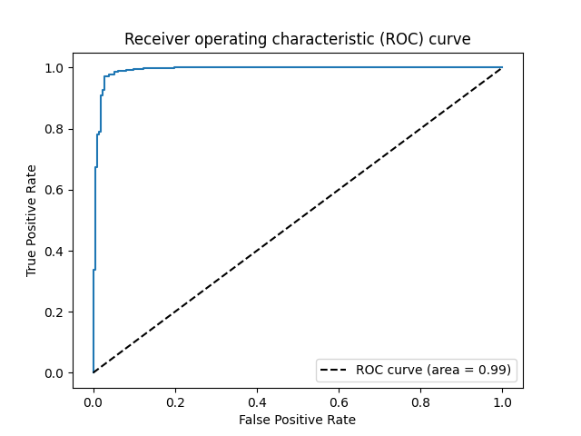
The output of the code reports the information of the polynomial features for the selected model among candidates, and its corresponding area under the curve (AUC), which is 0.99, indicating the selected model would have an admirable contribution in practice.

Moreover, the best choice of parameter combination is shown above: 2 degree with "self-combination", implying the inclusion of the pairwise interactions between any two features can lead to a better model generalization.

Here is its ROC curve:

import matplotlib.pyplot as plt
proba = grid_search.predict_proba(X)
fpr, tpr, _ = roc_curve(y, proba[:, 1])
plt.plot(fpr, tpr)
plt.plot([0, 1], [0, 1], 'k--', label="ROC curve (area = %0.2f)" % auc(fpr, tpr))
plt.xlabel('False Positive Rate')
plt.ylabel('True Positive Rate')
plt.title("Receiver operating characteristic (ROC) curve")
plt.legend(loc="lower right")
plt.show()

sphinx_gallery_thumbnail_path = 'Tutorial/figure/scikit_learn.png'