Note
Go to the end to download the full example code.
Linear Regression#
In this tutorial, we are going to demonstrate how to use the abess package to carry out best subset selection
in linear regression with both simulated data and real data.
Our package abess implements a polynomial algorithm in the following best-subset selection problem:
where \(\| \cdot \|_2\) is the \(\ell_2\) norm, \(\|\beta\|_0=\sum_{i=1}^pI( \beta_i\neq 0)\)
is the \(\ell_0\) norm of \(\beta\), and the sparsity level \(s\)
is an unknown non-negative integer to be determined.
Next, we present an example to show the abess package can get an optimal estimation.
Toward optimality: adaptive best-subset selection#
Synthetic dataset#
We generate a design matrix \(X\) containing \(n = 300\) observations and each observation has \(p = 1000\) predictors. The response variable \(y\) is linearly related to the first, second, and fifth predictors in \(X\):
where \(\epsilon\) is a standard normal random variable.
import numpy as np
from abess.datasets import make_glm_data
np.random.seed(0)

n = 300
p = 1000
true_support_set=[0, 1, 4]
true_coef = np.array([3, 1.5, 2])
real_coef = np.zeros(p)
real_coef[true_support_set] = true_coef
data1 = make_glm_data(n=n, p=p, k=len(true_coef), family="gaussian", coef_=real_coef)

print(data1.x.shape)
print(data1.y.shape)
(300, 1000)
(300,)
This dataset is high-dimensional and brings large challenge for subset selection.
As a typical data examples, it mimics data appeared in real-world for modern scientific researches and data mining,
and serves a good quick example for demonstrating the power of the abess library.
Optimality#
The optimality of subset selection means:
true_support_set(i.e.[0, 1, 4]) can be exactly identified;the estimated coefficients is ordinary least squares (OLS) estimator under the true subset such that is very closed to
true_coef = np.array([3, 1.5, 2]).
To understand the second criterion, we take a look on the estimation given by scikit-learn library:
from sklearn.linear_model import LinearRegression as SKLLinearRegression
sklearn_lr = SKLLinearRegression()
sklearn_lr.fit(data1.x[:, [0, 1, 4]], data1.y)
print("OLS estimator: ", sklearn_lr.coef_)
OLS estimator: [3.00085183 1.44388323 2.00633204]
The fitted coefficients sklearn_lr.coef_ is OLS estimator
when the true support set is known.
It is very closed to the true_coef, and is hard to be improve under finite sample size.
Adaptive Best Subset Selection#
The adaptive best subset selection (ABESS) algorithm is a very powerful for the selection of the best subset. We will illustrate its power by showing it can reach to the optimality.
The following code shows the simple syntax for using ABESS algorithm via abess library.
from abess import LinearRegression
model = LinearRegression()
model.fit(data1.x, data1.y)
LinearRegression functions in abess is designed for selecting the best subset under the linear model,
which can be imported by: from abess import LinearRegression.
Following similar syntax like scikit-learn, we can fit the data via ABESS algorithm.
Next, we going to see that the above approach can successfully recover the true set np.array([0, 1, 4]).
The fitted coefficients are stored in model.coef_.
We use np.nonzero function to find the selected subset of abess,
and we can extract the non-zero entries in model.coef_ which is the coefficients estimation for the selected predictors.
ind = np.nonzero(model.coef_)
print("estimated non-zero: ", ind)
print("estimated coef: ", model.coef_[ind])
estimated non-zero:  (array([0, 1, 4]),)
estimated coef:  [3.00085183 1.44388323 2.00633204]
From the result, we know that abess exactly found the true set np.array([0, 1, 4]) among all 1000 predictors.
Besides, the estimated coefficients of them are quite close to the real ones,
and is exactly the same as the estimation sklearn_lr.coef_ given by scikit-learn.
Real data example#
Hitters Dataset#
Now we focus on real data on the Hitters dataset. We hope to use several predictors related to the performance of the baseball athletes last year to predict their salary.
First, let's have a look at this dataset. There are 19 variables except Salary and 322 observations.
import os
import pandas as pd

data2 = pd.read_csv(os.path.join(os.getcwd(), 'Hitters.csv'))
print(data2.shape)
print(data2.head(5))
(322, 20)
   AtBat  Hits  HmRun  Runs  RBI  ...  PutOuts  Assists  Errors  Salary  NewLeague
0    293    66      1    30   29  ...      446       33      20     NaN          A
1    315    81      7    24   38  ...      632       43      10   475.0          N
2    479   130     18    66   72  ...      880       82      14   480.0          A
3    496   141     20    65   78  ...      200       11       3   500.0          N
4    321    87     10    39   42  ...      805       40       4    91.5          N

[5 rows x 20 columns]
Since the dataset contains some missing values, we simply drop those rows with missing values. Then we have 263 observations remain:
data2 = data2.dropna()
print(data2.shape)
(263, 20)
What is more, before fitting, we need to transfer the character variables to dummy variables:
data2 = pd.get_dummies(data2)
data2 = data2.drop(['League_A', 'Division_E', 'NewLeague_A'], axis=1)
print(data2.shape)
print(data2.head(5))
(263, 20)
   AtBat  Hits  HmRun  Runs  ...  Salary  League_N  Division_W  NewLeague_N
1    315    81      7    24  ...   475.0      True        True         True
2    479   130     18    66  ...   480.0     False        True        False
3    496   141     20    65  ...   500.0      True       False         True
4    321    87     10    39  ...    91.5      True       False         True
5    594   169      4    74  ...   750.0     False        True        False

[5 rows x 20 columns]
Model Fitting#
As what we do in simulated data, an adaptive best subset can be formed easily:
The result can be shown as follows:
ind = np.nonzero(model.coef_)
print("non-zero:\n", data2.columns[ind])
print("coef:\n", model.coef_)
non-zero:
 Index(['Hits', 'CRBI', 'PutOuts', 'League_N'], dtype='object')
coef:
 [   0.            2.67579779    0.            0.            0.
    0.            0.            0.            0.            0.
    0.            0.681779      0.            0.27350022    0.
    0.            0.         -139.9538855     0.        ]
Automatically, variables Hits, CHits, CHmRun, PutOuts, League_N are chosen in the model (the chosen sparsity level is 5).
More on the results#
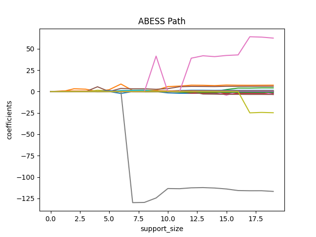
We can also plot the path of abess process:
import matplotlib.pyplot as plt
coef = np.zeros((20, 19))
ic = np.zeros(20)
for s in range(20):
    model = LinearRegression(support_size=s)
    model.fit(x, y)
    coef[s, :] = model.coef_
    ic[s] = model.eval_loss_

for i in range(19):
    plt.plot(coef[:, i], label=i)

plt.xlabel('support_size')
plt.ylabel('coefficients')
plt.title('ABESS Path')
plt.show()
Besides, we can also generate a graph about the tuning parameter. Remember that we used the default EBIC to tune the support size.
plt.plot(ic, 'o-')
plt.xlabel('support_size')
plt.ylabel('EBIC')
plt.title('Model selection via EBIC')
plt.show()
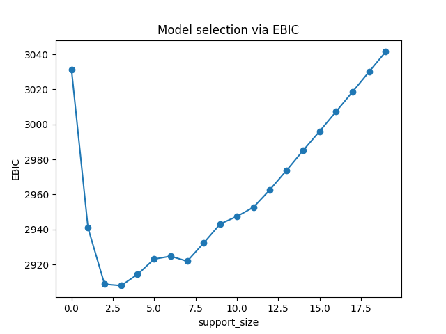
In EBIC criterion, a subset with the support size 4 has the lowest value, so the process adaptively chooses 4 variables. Note that under other information criteria, the result may be different.
R tutorial#
For R tutorial, please view https://abess-team.github.io/abess/articles/v01-abess-guide.html.
Total running time of the script: (0 minutes 1.275 seconds)