Note
Go to the end to download the full example code.
Classification: Logistic Regression and Beyond#
We would like to use an example to show how the best subset selection for logistic regression works in our program.
Real Data Example#
Titanic Dataset#
Consider the Titanic dataset obtained from the Kaggle competition: https://www.kaggle.com/c/titanic/data. The dataset consists of data of 889 passengers, and the goal of the competition is to predict the survival status (yes/no) based on features including the class of service, the sex, the age, etc.
import pandas as pd

dt = pd.read_csv("train.csv")
print(dt.head(5))
   PassengerId  Survived  Pclass  ...     Fare Cabin  Embarked
0            1         0       3  ...   7.2500   NaN         S
1            2         1       1  ...  71.2833   C85         C
2            3         1       3  ...   7.9250   NaN         S
3            4         1       1  ...  53.1000  C123         S
4            5         0       3  ...   8.0500   NaN         S

[5 rows x 12 columns]
We only focus on some numerical or categorical variables:
predictor variables: Pclass, Sex, Age, SibSp, Parch, Fare, Embarked;
response variable is Survived.
dt = dt.iloc[:, [1, 2, 4, 5, 6, 7, 9, 11]]  # variables interested
dt['Pclass'] = dt['Pclass'].astype(str)
print(dt.head(5))
   Survived Pclass     Sex   Age  SibSp  Parch     Fare Embarked
0         0      3    male  22.0      1      0   7.2500        S
1         1      1  female  38.0      1      0  71.2833        C
2         1      3  female  26.0      0      0   7.9250        S
3         1      1  female  35.0      1      0  53.1000        S
4         0      3    male  35.0      0      0   8.0500        S
However, some rows contain missing values (NaN) and we need to drop them.
dt = dt.dropna()
print('sample size: ', dt.shape)
sample size: (712, 8)
Then use dummy variables to replace classification variables:
dt1 = pd.get_dummies(dt)
print(dt1.head(5))
   Survived   Age  SibSp  Parch  ...  Sex_male  Embarked_C  Embarked_Q  Embarked_S
0         0  22.0      1      0  ...      True       False       False        True
1         1  38.0      1      0  ...     False        True       False       False
2         1  26.0      0      0  ...     False       False       False        True
3         1  35.0      1      0  ...     False       False       False        True
4         0  35.0      0      0  ...      True       False       False        True

[5 rows x 13 columns]
Now we split dt1 into training set and testing set:
from sklearn.model_selection import train_test_split
import numpy as np

X = np.array(dt1.drop('Survived', axis=1))
Y = np.array(dt1.Survived)

train_x, test_x, train_y, test_y = train_test_split(
    X, Y, test_size=0.33, random_state=0)
print('train size: ', train_x.shape[0])
print('test size:', test_x.shape[0])
train size:  477
test size: 235
Here train_x contains:
V0: dummy variable, 1st ticket class (1-yes, 0-no)
V1: dummy variable, 2nd ticket class (1-yes, 0-no)
V2: dummy variable, sex (1-male, 0-female)
V3: Age
V4: # of siblings / spouses aboard the Titanic
V5: # of parents / children aboard the Titanic
V6: Passenger fare
V7: dummy variable, Cherbourg for embarkation (1-yes, 0-no)
V8: dummy variable, Queenstown for embarkation (1-yes, 0-no)
And train_y indicates whether the passenger survived (1-yes, 0-no).
train_x:
 [[54.0 1 0 59.4 True False False True False True False False]
 [30.0 0 0 8.6625 False False True True False False False True]
 [47.0 0 0 38.5 True False False False True False False True]
 [28.0 2 0 7.925 False False True False True False False True]
 [29.0 1 0 26.0 False True False True False False False True]]
train_y:
 [1 0 0 0 1]
Model Fitting#
The LogisticRegression() function in the abess.linear allows us to perform
best subset selection in a highly efficient way.
For example, in the Titanic sample, if you want to look for a best subset with no more than 5 variables
on the logistic model, you can call:
from abess import LogisticRegression

s = 5   # max target sparsity
model = LogisticRegression(support_size=range(0, s + 1))
model.fit(train_x, train_y)
Now the model.coef_ contains the coefficients of logistic model with no more than 5 variables.
That is, those variables with a coefficient 0 is unused in the model:
print(model.coef_)
[-0.05410776 -0.53642966  0.          0.          1.74091231  0.
 -1.26223831  2.7096497   0.          0.          0.          0.        ]
By default, the LogisticRegression function set support_size = range(0, min(p,n/log(n)p)
and the best support size is determined by the Extended Bayesian Information Criteria (EBIC).
You can change the tuning criterion by specifying the argument ic_type.
The available tuning criteria now are "gic", "aic", "bic", "ebic".
For a quicker solution, you can change the tuning strategy to a golden section path which tries to find the elbow point of the tuning criterion over the hyperparameter space. Here we give an example.
model_gs = LogisticRegression(path_type="gs", s_min=0, s_max=s)
model_gs.fit(train_x, train_y)
print(model_gs.coef_)
[-0.05410776 -0.53642966  0.          0.          1.74091231  0.
 -1.26223831  2.7096497   0.          0.          0.          0.        ]
where s_min and s_max bound the support size and this model gives the same answer as before.
More on the Results#
After fitting with model.fit(), we can further do more exploring work to interpret it.
As we show above, model.coef_ contains the sparse coefficients of variables and
those non-zero values indicate "important" variables chosen in the model.
print('Intercept: ', model.intercept_)
print('coefficients: \n', model.coef_)
print('Used variables\' index:', np.nonzero(model.coef_ != 0)[0])
Intercept:  0.5742977507847967
coefficients:
 [-0.05410776 -0.53642966  0.          0.          1.74091231  0.
 -1.26223831  2.7096497   0.          0.          0.          0.        ]
Used variables' index: [0 1 4 6 7]
The training loss and the score under information criterion:
print('Training Loss: ', model.train_loss_)
print('IC: ', model.eval_loss_)
Training Loss:  204.35270048059672
IC:  464.39204991351517
Prediction is allowed for the estimated model. Just call
model.predict() function like:
[0 0 1 0 0 0 1 0 0 1 1 1 1 0 0 1 0 1 0 0 0 1 1 0 1 0 0 0 1 0 0 0 0 1 1 1 1
 1 0 0 0 0 0 0 0 0 1 0 0 1 1 1 1 0 1 1 0 0 1 0 0 0 0 0 0 0 1 0 1 1 0 1 1 1
 0 1 0 0 0 0 1 1 0 1 1 0 0 0 1 0 0 0 1 1 1 0 1 1 0 0 0 1 0 0 0 0 1 0 0 0 0
 1 1 0 0 0 0 0 0 0 0 0 0 1 0 0 0 0 1 1 0 1 1 1 1 1 1 0 0 0 0 0 1 1 1 0 0 0
 0 0 0 0 1 1 1 0 0 1 1 1 1 0 1 1 0 0 0 0 0 0 1 1 1 0 1 1 1 0 0 0 0 0 0 0 0
 1 0 0 1 1 0 1 1 0 1 1 0 0 1 1 0 1 0 1 0 0 0 0 0 0 1 1 1 1 0 0 1 1 0 1 1 0
 0 1 0 0 0 0 0 0 0 0 0 0 0]
Besides, we can also call for the survival probability of each observation by model.predict_proba(),
which returns a matrix with two columns. The first column corresponds to probability for class "0", and
the second is for class "1" (survived).
Then, we tend to classify the observation into more likely class.
[[0.50743387 0.49256613]
 [0.74057032 0.25942968]
 [0.15071537 0.84928463]
 [0.79795817 0.20204183]
 [0.96198452 0.03801548]
 [0.95977651 0.04022349]
 [0.27648557 0.72351443]
 [0.76884378 0.23115622]
 [0.76884378 0.23115622]
 [0.33165327 0.66834673]
 [0.03224465 0.96775535]
 [0.35094054 0.64905946]
 [0.01538079 0.98461921]
 [0.84761133 0.15238867]
 [0.74995921 0.25004079]
 [0.42359788 0.57640212]
 [0.73004032 0.26995968]
 [0.28735418 0.71264582]
 [0.62208165 0.37791835]
 [0.8228686  0.1771314 ]
 [0.74226703 0.25773297]
 [0.24607858 0.75392142]
 [0.12025589 0.87974411]
 [0.59748431 0.40251569]
 [0.43558118 0.56441882]
 [0.65942131 0.34057869]
 [0.77994844 0.22005156]
 [0.932841   0.067159  ]
 [0.42119469 0.57880531]
 [0.66352233 0.33647767]
 [0.84344878 0.15655122]
 [0.97317339 0.02682661]
 [0.85446957 0.14553043]
 [0.30336212 0.69663788]
 [0.10921555 0.89078445]
 [0.12074848 0.87925152]
 [0.08073996 0.91926004]
 [0.40918613 0.59081387]
 [0.57002721 0.42997279]
 [0.54346526 0.45653474]
 [0.61153036 0.38846964]
 [0.90979818 0.09020182]
 [0.94257539 0.05742461]
 [0.92226281 0.07773719]
 [0.9005148  0.0994852 ]
 [0.88993666 0.11006334]
 [0.0180426  0.9819574 ]
 [0.85780137 0.14219863]
 [0.8903911  0.1096089 ]
 [0.03059829 0.96940171]
 [0.28648812 0.71351188]
 [0.30336212 0.69663788]
 [0.36336243 0.63663757]
 [0.74057032 0.25942968]
 [0.45021417 0.54978583]
 [0.46690207 0.53309793]
 [0.92967528 0.07032472]
 [0.9293708  0.0706292 ]
 [0.13110112 0.86889888]
 [0.62098833 0.37901167]
 [0.56123326 0.43876674]
 [0.96915459 0.03084541]
 [0.85446957 0.14553043]
 [0.80006385 0.19993615]
 [0.70819044 0.29180956]
 [0.88171401 0.11828599]
 [0.05413855 0.94586145]
 [0.69389487 0.30610513]
 [0.01236779 0.98763221]
 [0.19088286 0.80911714]
 [0.74057032 0.25942968]
 [0.06948297 0.93051703]
 [0.0902975  0.9097025 ]
 [0.48714638 0.51285362]
 [0.95075583 0.04924417]
 [0.46234646 0.53765354]
 [0.51757961 0.48242039]
 [0.73959052 0.26040948]
 [0.90525825 0.09474175]
 [0.6615436  0.3384564 ]
 [0.44892685 0.55107315]
 [0.11974729 0.88025271]
 [0.90941602 0.09058398]
 [0.18266554 0.81733446]
 [0.13163148 0.86836852]
 [0.90525825 0.09474175]
 [0.95538456 0.04461544]
 [0.71924495 0.28075505]
 [0.21109988 0.78890012]
 [0.86106974 0.13893026]
 [0.97565829 0.02434171]
 [0.95302055 0.04697945]
 [0.29853147 0.70146853]
 [0.08595031 0.91404969]
 [0.33767709 0.66232291]
 [0.9005148  0.0994852 ]
 [0.06280397 0.93719603]
 [0.1577817  0.8422183 ]
 [0.8903911  0.1096089 ]
 [0.84530315 0.15469685]
 [0.84761133 0.15238867]
 [0.14120978 0.85879022]
 [0.77994844 0.22005156]
 [0.75908805 0.24091195]
 [0.78831956 0.21168044]
 [0.84761133 0.15238867]
 [0.39506122 0.60493878]
 [0.67355065 0.32644935]
 [0.73874787 0.26125213]
 [0.92482907 0.07517093]
 [0.86106974 0.13893026]
 [0.25965364 0.74034636]
 [0.15253925 0.84746075]
 [0.54786818 0.45213182]
 [0.9293708  0.0706292 ]
 [0.74057032 0.25942968]
 [0.77994844 0.22005156]
 [0.98164302 0.01835698]
 [0.85836737 0.14163263]
 [0.79788631 0.20211369]
 [0.84761133 0.15238867]
 [0.90009763 0.09990237]
 [0.76081454 0.23918546]
 [0.26927389 0.73072611]
 [0.73784984 0.26215016]
 [0.96391455 0.03608545]
 [0.96129876 0.03870124]
 [0.83746312 0.16253688]
 [0.25965364 0.74034636]
 [0.02006328 0.97993672]
 [0.91829389 0.08170611]
 [0.35926408 0.64073592]
 [0.15966607 0.84033393]
 [0.14789964 0.85210036]
 [0.19016604 0.80983396]
 [0.02742217 0.97257783]
 [0.36336243 0.63663757]
 [0.98180978 0.01819022]
 [0.95478642 0.04521358]
 [0.88499785 0.11500215]
 [0.64716682 0.35283318]
 [0.9395756  0.0604244 ]
 [0.19016604 0.80983396]
 [0.34572827 0.65427173]
 [0.43558118 0.56441882]
 [0.78909413 0.21090587]
 [0.90979818 0.09020182]
 [0.84761133 0.15238867]
 [0.90794231 0.09205769]
 [0.86741702 0.13258298]
 [0.92967528 0.07032472]
 [0.89556126 0.10443874]
 [0.32670564 0.67329436]
 [0.08952309 0.91047691]
 [0.12858887 0.87141113]
 [0.86741702 0.13258298]
 [0.86106974 0.13893026]
 [0.30998425 0.69001575]
 [0.0145825  0.9854175 ]
 [0.25965364 0.74034636]
 [0.04842691 0.95157309]
 [0.90009763 0.09990237]
 [0.02115516 0.97884484]
 [0.48933053 0.51066947]
 [0.95558225 0.04441775]
 [0.95558225 0.04441775]
 [0.71638648 0.28361352]
 [0.96512977 0.03487023]
 [0.50511029 0.49488971]
 [0.8821979  0.1178021 ]
 [0.35926408 0.64073592]
 [0.37487948 0.62512052]
 [0.02115516 0.97884484]
 [0.9293708  0.0706292 ]
 [0.49506961 0.50493039]
 [0.37596932 0.62403068]
 [0.13163148 0.86836852]
 [0.86106974 0.13893026]
 [0.82544239 0.17455761]
 [0.6968841  0.3031159 ]
 [0.92226281 0.07773719]
 [0.62098833 0.37901167]
 [0.88221559 0.11778441]
 [0.5298741  0.4701259 ]
 [0.59737712 0.40262288]
 [0.0630781  0.9369219 ]
 [0.82544239 0.17455761]
 [0.83310188 0.16689812]
 [0.33359333 0.66640667]
 [0.12661189 0.87338811]
 [0.75738401 0.24261599]
 [0.41474865 0.58525135]
 [0.23939759 0.76060241]
 [0.90941602 0.09058398]
 [0.041657   0.958343  ]
 [0.27018941 0.72981059]
 [0.69488121 0.30511879]
 [0.70819044 0.29180956]
 [0.22574405 0.77425595]
 [0.03224465 0.96775535]
 [0.9141412  0.0858588 ]
 [0.13163148 0.86836852]
 [0.96915459 0.03084541]
 [0.28099043 0.71900957]
 [0.91273698 0.08726302]
 [0.94704734 0.05295266]
 [0.65133737 0.34866263]
 [0.67146626 0.32853374]
 [0.965596   0.034404  ]
 [0.84049023 0.15950977]
 [0.08914497 0.91085503]
 [0.47466173 0.52533827]
 [0.19863876 0.80136124]
 [0.44777727 0.55222273]
 [0.92605446 0.07394554]
 [0.75082977 0.24917023]
 [0.23524154 0.76475846]
 [0.26568554 0.73431446]
 [0.72817106 0.27182894]
 [0.1023766  0.8976234 ]
 [0.32670564 0.67329436]
 [0.95558225 0.04441775]
 [0.69875031 0.30124969]
 [0.02351608 0.97648392]
 [0.83746312 0.16253688]
 [0.85107278 0.14892722]
 [0.97930718 0.02069282]
 [0.71732988 0.28267012]
 [0.94257539 0.05742461]
 [0.94987806 0.05012194]
 [0.87351692 0.12648308]
 [0.93254923 0.06745077]
 [0.91724157 0.08275843]
 [0.90979818 0.09020182]
 [0.932841   0.067159  ]]
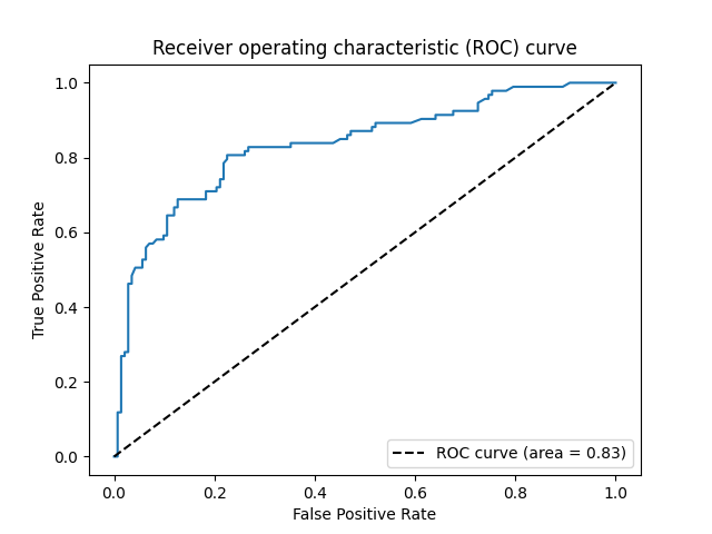
We can also generate an ROC curve and calculate tha AUC value. On this dataset, the AUC is 0.83, which is rather desirable.
from sklearn.metrics import roc_curve, auc
import matplotlib.pyplot as plt

fpr, tpr, _ = roc_curve(test_y, fitted_p[:, 1])
plt.plot(fpr, tpr)
plt.plot([0, 1], [0, 1], 'k--', label="ROC curve (area = %0.2f)" % auc(fpr, tpr))
plt.xlabel('False Positive Rate')
plt.ylabel('True Positive Rate')
plt.title("Receiver operating characteristic (ROC) curve")
plt.legend(loc="lower right")
plt.show()
Extension: Multi-class Classification#
Multinomial logistic regression#
When the number of classes is more than 2, we call it multi-class classification task. Logistic regression can be extended to model several classes of events such as determining whether an image contains a cat, dog, lion, etc. Each object being detected in the image would be assigned a probability between 0 and 1, with a sum of one. The extended model is multinomial logistic regression.
To arrive at the multinomial logistic model, one can imagine, for \(K\) possible classes, running \(K−1\) independent logistic regression models, in which one class is chosen as a "pivot" and then the other \(K−1\) classes are separately regressed against the pivot outcome. This would proceed as follows, if class \(K\) (the last outcome) is chosen as the pivot:
Then, the probability to choose the \(j\)-th class can be easily derived to be:
and subsequently, we would that the object belongs to the \(j^*\)-th class if the \(j^*=\arg\max_j \mathbb{P}(y=j)\). Notice that, for \(K\) possible classes case, there are \(p\times(K−1)\) unknown parameters: \(\beta^{(1)},\dots,\beta^{(K−1)}\) to be estimated. Because the number of parameters increases as \(K\), it is even more urgent to constrain the model complexity. And the best subset selection for multinomial logistic regression aims to maximize the log-likelihood function and control the model complexity by restricting \(B=(\beta^{(1)},\dots,\beta^{(K−1)})\) with \(||B||_{0,2}\leq s\) where \(||B||_{0,2}=\sum_{i=1}^p I(B_{i\cdot}=0)\), \(B_{i\cdot}\) is the \(i\)-th row of coefficient matrix \(B\) and \(0\in \mathbb{R}^{K-1}\) is an all zero vector. In other words, each row of \(B\) would be either all zero or all non-zero.
Simulated Data Example#
We shall conduct Multinomial logistic regression on an artificial dataset for demonstration.
The make_multivariate_glm_data() provides a simple way to generate suitable dataset for this task.
The assumption behind this model is that the response vector follows a multinomial distribution. The artificial dataset contains 100 observations and 20 predictors but only five predictors have influence on the three possible classes.
from abess.datasets import make_multivariate_glm_data

n = 100  # sample size
p = 20  # all predictors
k = 5   # real predictors
M = 3   # number of classes

np.random.seed(0)
dt = make_multivariate_glm_data(n=n, p=p, k=k, family="multinomial", M=M)
print(dt.coef_)
print('real variables\' index:\n', set(np.nonzero(dt.coef_)[0]))
[[ 0.          0.          0.        ]
 [ 0.          0.          0.        ]
 [ 1.09734231  4.03598978  0.        ]
 [ 0.          0.          0.        ]
 [ 0.          0.          0.        ]
 [ 9.91227834 -3.47987303  0.        ]
 [ 0.          0.          0.        ]
 [ 0.          0.          0.        ]
 [ 0.          0.          0.        ]
 [ 0.          0.          0.        ]
 [ 8.93282229  8.93249765  0.        ]
 [-4.03426165 -2.70336848  0.        ]
 [ 0.          0.          0.        ]
 [ 0.          0.          0.        ]
 [ 0.          0.          0.        ]
 [ 0.          0.          0.        ]
 [ 0.          0.          0.        ]
 [ 0.          0.          0.        ]
 [-5.53475149 -2.65928982  0.        ]
 [ 0.          0.          0.        ]]
real variables' index:
 {2, 5, 10, 11, 18}
To carry out best subset selection for multinomial logistic regression,
we can call the MultinomialRegression(). Here is an example.
from abess import MultinomialRegression

s = 5
model = MultinomialRegression(support_size=range(0, s + 1))
model.fit(dt.x, dt.y)
Its use is quite similar to LogisticRegression. We can get the
coefficients to recognize "in-model" variables.
print('intercept:\n', model.intercept_)
print('coefficients:\n', model.coef_)
intercept:
 [0.78190717 1.22272385 0.        ]
coefficients:
 [[ 0.          0.          0.        ]
 [ 0.          0.          0.        ]
 [ 1.03856319  3.4493283   0.        ]
 [ 0.          0.          0.        ]
 [ 0.          0.          0.        ]
 [ 6.65426538 -4.29362189  0.        ]
 [ 0.          0.          0.        ]
 [ 0.          0.          0.        ]
 [ 0.          0.          0.        ]
 [ 0.          0.          0.        ]
 [ 7.42869845  7.89026858  0.        ]
 [-3.90706745 -3.07155561  0.        ]
 [ 0.          0.          0.        ]
 [ 0.          0.          0.        ]
 [ 0.          0.          0.        ]
 [ 0.          0.          0.        ]
 [ 0.          0.          0.        ]
 [ 0.          0.          0.        ]
 [-3.37430731 -0.61106365  0.        ]
 [ 0.          0.          0.        ]]
So those variables used in model can be recognized and we can find that they are the same as the data's "real" coefficients we generate.
print('used variables\' index:\n', set(np.nonzero(model.coef_)[0]))
used variables' index:
 {2, 5, 10, 11, 18}
The abess R package also supports classification tasks.
For R tutorial, please view
https://abess-team.github.io/abess/articles/v03-classification.html.
Total running time of the script: (0 minutes 0.180 seconds)