Work with scikit-learn

abess is very easy to work with the famous package scikit-learn, and here is an example. We going to illustrate the integration of the abess with scikit-learn’s pre-processing and model selection modules to build a non-linear model for diagnosing malignant tumors. Let start with importing necessary dependencies:

import numpy as np
from abess.datasets import make_glm_data
from abess.linear import LinearRegression, LogisticRegression
from sklearn.datasets import fetch_openml, load_breast_cancer
from sklearn.pipeline import Pipeline, make_pipeline
from sklearn.metrics import roc_auc_score, make_scorer, roc_curve, auc
from sklearn.compose import ColumnTransformer
from sklearn.preprocessing import MinMaxScaler, OneHotEncoder, PolynomialFeatures, StandardScaler
from sklearn.model_selection import GridSearchCV, TimeSeriesSplit, cross_val_score
from sklearn.feature_selection import SelectFromModel

Establish the process

Suppose we would like to extend the original variables to their interactions, and then do LogisticRegression on them. This can be record with Pipeline:

pipe = Pipeline([
    ('poly', PolynomialFeatures(include_bias=False)),   # without intercept
    ('standard', StandardScaler()),
    ('alogistic', LogisticRegression())
])

Parameter grid

We can give different parameters to model and let the program choose the best. Here we should give parameters for PolynomialFeatures, for example:

param_grid = {
    # whether the "self-combination" (e.g. X^2, X^3) exists
    'poly__interaction_only': [True, False],
    'poly__degree': [1, 2, 3]                   # the degree of polynomial
}

Note that the program would try all combinations of what we give, which means that there are \(2\times3=6\) combinations of parameters will be tried.

Criterion

After giving a grid of parameters, we should define what is a "better" result. For example, the AUC (area under ROC curve) can be a criterion and the larger, the better.

scorer = make_scorer(roc_auc_score, greater_is_better=True)

Cross Validation

For more accurate results, cross validation (CV) is often formed.

Suppose that the data is independent and identically distributed (i.i.d.) that all samples stem from the same generative process and that the generative process has no memory of past generated samples. A typical CV strategy is K-fold and a corresponding grid search procedure can be made as follows:

grid_search = GridSearchCV(pipe, param_grid, scoring=scorer, cv=5)

However, if there exists correlation between observations (e.g. time-series data), K-fold strategy is not appropriate any more. An alternative CV strategy is TimeSeriesSplit. It is a variation of K-fold which returns first K folds as train set and the (K+1)-th fold as test set.

The following example shows a combinatioon of abess and TimeSeriesSplit applied to Bike_Sharing_Demand dataset and it returns the cv score of a specific choice of support_size.

bike_sharing = fetch_openml('Bike_Sharing_Demand', version=2, as_frame=True)
df = bike_sharing.frame
X = df.drop('count', axis='columns')
y = df['count'] / df['count'].max()

ts_cv = TimeSeriesSplit(
    n_splits=5,
    gap=48,
    max_train_size=10000,
    test_size=1000,
)

categorical_columns = ['weather', 'season', 'holiday', 'workingday',]
one_hot_encoder = OneHotEncoder(handle_unknown='ignore')

one_hot_abess_pipeline = make_pipeline(
    ColumnTransformer(
        transformers=[
            ('categorical', one_hot_encoder, categorical_columns),
            ('one_hot_time', one_hot_encoder, ['hour', 'weekday', 'month']),
        ],
        remainder=MinMaxScaler(),
    ),
    LinearRegression(support_size=5),
)

scores = cross_val_score(one_hot_abess_pipeline, X, y, cv=ts_cv)
print("%0.2f score with a standard deviation of %0.2f" % (scores.mean(), scores.std()))

0.21 score with a standard deviation of 0.06

Model fitting

Eveything is prepared now. We can simply load the data and put it into grid_search:

X, y = load_breast_cancer(return_X_y=True)
grid_search.fit(X, y)
print([grid_search.best_score_, grid_search.best_params_])

[0.9714645755670978, {'poly__degree': 2, 'poly__interaction_only': True}]

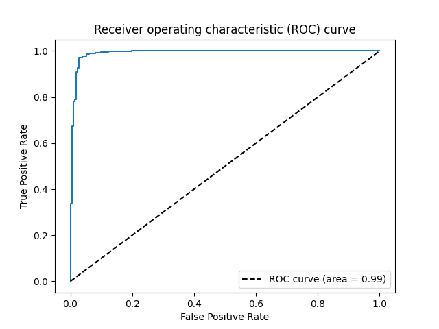
The output of the code reports the information of the polynomial features for the selected model among candidates, and its corresponding area under the curve (AUC), which is over 0.97, indicating the selected model would have an admirable contribution in practice.

Moreover, the best choice of parameter combination is shown above: 2 degree with "self-combination", implying the inclusion of the pairwise interactions between any two features can lead to a better model generalization.

Here is its ROC curve:

import matplotlib.pyplot as plt
proba = grid_search.predict_proba(X)
fpr, tpr, _ = roc_curve(y, proba[:, 1])
plt.plot(fpr, tpr)
plt.plot([0, 1], [0, 1], 'k--', label="ROC curve (area = %0.2f)" % auc(fpr, tpr))
plt.xlabel('False Positive Rate')
plt.ylabel('True Positive Rate')
plt.title("Receiver operating characteristic (ROC) curve")
plt.legend(loc="lower right")
plt.show()

Feature selection

Besides being used to make prediction explicitly, abess can be exploited to select important features. The following example shows how to perform abess-based feature selection using sklearn.feature_selection.SelectFromModel.

np.random.seed(0)
n, p, k = 300, 1000, 5
data = make_glm_data(n=n, p=p, k=k, family='gaussian')
X, y = data.x, data.y
print('Shape of original data: ', X.shape)

model = LinearRegression().fit(X, y)
sfm = SelectFromModel(model, prefit=True)
X_new = sfm.transform(X)
print('Shape of transformed data: ', X_new.shape)

Shape of original data:  (300, 1000)
Shape of transformed data:  (300, 5)

sphinx_gallery_thumbnail_path = 'Tutorial/figure/scikit_learn.png'