Positive Responses: Poisson & Gamma Regressions

Poisson Regression

Poisson Regression involves regression models in which the response variable is in the form of counts. For example, the count of number of car accidents or number of customers in line at a reception desk. The response variables is assumed to follow a Poisson distribution.

The general mathematical equation for Poisson regression is

\[\log(E(y)) = \beta_0 + \beta_1 X_1+\beta_2 X_2+\dots+\beta_p X_p.\]

Simulated Data Example

We generate some artificial data using this logic. Consider a dataset containing n=100 observations with p=6 variables. The make_glm_data() function allows uss to generate simulated data. By specifying k = 3, we set only 3 of the 6 variables to have effect on the expectation of the response.

import numpy as np
from abess.datasets import make_glm_data
np.random.seed(0)

n = 100
p = 6
k = 3
data = make_glm_data(n=n, p=p, k=k, family="poisson")
print("the first 5 x observation:\n", data.x[0:5, ])
print("the first 5 y observation:\n", data.y[0:5])

the first 5 x observation:
 [[ 0.11025327  0.02500983  0.06117112  0.14005582  0.11672237 -0.06107987]
 [ 0.05938053 -0.00945983 -0.00645118  0.02566241  0.00900272  0.09089209]
 [ 0.04756486  0.00760469  0.02774145  0.02085465  0.09337994 -0.01282239]
 [ 0.01956673 -0.05338098 -0.15956186  0.04085116  0.05402726 -0.04638531]
 [ 0.14185966 -0.09089785  0.00285991 -0.01169899  0.0957987   0.09183492]]
the first 5 y observation:
 [0 0 0 0 0]

Notice that, the response have non-negative integer value.

The effective predictors and real coefficients are:

print("non-zero:\n", np.nonzero(data.coef_))
print("real coef:\n", data.coef_)

non-zero:
 (array([0, 2, 5]),)
real coef:
 [-9.28248323  0.         -8.95444082  0.          0.          4.85973384]

Model Fitting

The PoissonRegression() function in the abess package allows you to perform best subset selection in a highly efficient way. We can call the function using formula like:

from abess.linear import PoissonRegression

model = PoissonRegression(support_size=range(7))
model.fit(data.x, data.y)

PoissonRegression(support_size=range(0, 7))

In a Jupyter environment, please rerun this cell to show the HTML representation or trust the notebook.
On GitHub, the HTML representation is unable to render, please try loading this page with nbviewer.org.

where support_size contains the level of sparsity we consider, and the program can adaptively choose the "best" one. The result of coefficients can be viewed through model.coef_:

print(model.coef_)

[-11.26494228   0.          -8.28071518   0.           0.
   7.2757849 ]

So that the first, third and last variables are thought to be useful in the model (the chosen sparsity is 3), which is the same as "real" variables. What's more, the predicted coefficients are also close to the real ones.

More on the Results

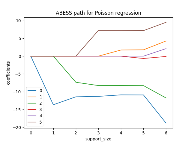
Actually, we can also plot the path of coefficients in abess process. This can be computed by fixing the support_size as one number from 0 to 6 each time:

import matplotlib.pyplot as plt

coef = np.zeros((7, 6))
ic = np.zeros(7)
for s in range(7):
    model = PoissonRegression(support_size=s)
    model.fit(data.x, data.y)
    coef[s, :] = model.coef_
    ic[s] = model.eval_loss_

for i in range(6):
    plt.plot(coef[:, i], label=i)

plt.xlabel('support_size')
plt.ylabel('coefficients')
plt.title('ABESS path for Poisson regression')
plt.legend()
plt.show()

And the evolution of information criterion (by default, we use EBIC):

plt.plot(ic, 'o-')
plt.xlabel('support_size')
plt.ylabel('EBIC')
plt.title('Model selection via EBIC')
plt.show()

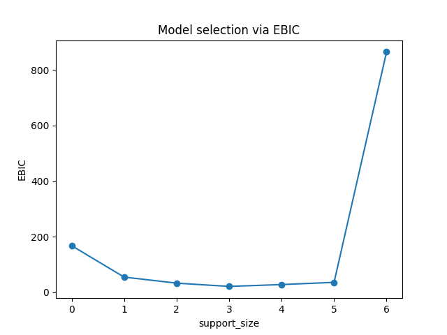
The lowest point is shown on support_size=3 and that's why the program chooses 3 variables as output.

Gamma Regression

Gamma regression can be used when you have positive continuous response variables such as payments for insurance claims, or the lifetime of a redundant system. It is well known that the density of Gamma distribution can be represented as a function of a mean parameter (\(\mu\)) and a shape parameter (\(\alpha\)), respectively,

\[f(y \mid \mu, \alpha)=\frac{1}{y \Gamma(\alpha)}\left(\frac{\alpha y}{\mu}\right)^{\alpha} e^{-\alpha y / \mu} {I}_{(0, \infty)}(y),\]

where \(I(\cdot)\) denotes the indicator function. In the Gamma regression model, response variables are assumed to follow Gamma distributions. Specifically,

\[y_i \sim Gamma(\mu_i, \alpha),\]

where \(-1/\mu_i = x_i^T\beta\).

Compared with Poisson regression, this time we consider the response variables as (continuous) levels of satisfaction.

Simulated Data Example

Firstly, we also generate data from make_glm_data(), but family = "gamma" is given this time:

np.random.seed(1)

n = 100
p = 6
k = 3
data = make_glm_data(n=n, p=p, k=k, family="gamma")
print("the first 5 x:\n", data.x[0:5, ])
print("the first 5 y:\n", data.y[0:5])

the first 5 x:
 [[ 0.10152159 -0.03823478 -0.03301073 -0.06706054  0.05408798 -0.14384617]
 [ 0.10905074 -0.04757543  0.01993994 -0.01558565  0.09138175 -0.12875879]
 [-0.02015108 -0.0240034   0.07086059 -0.0687432  -0.01077676 -0.05486615]
 [ 0.00263836  0.03642595 -0.0687887   0.07154523  0.05634942  0.0314059 ]
 [ 0.0563035  -0.04273299 -0.00768064 -0.05848559 -0.016743    0.03314722]]
the first 5 y:
 [0.04452499 0.0771034  0.05469221 0.03511288 0.0241431 ]

Notice that the response y is positive continuous value, which is different from the Poisson regression for integer value.

The effective predictors and their effects are presented below:

nnz_ind = np.nonzero(data.coef_)
print("non-zero:\n", nnz_ind)
print("non-zero coef:\n", data.coef_[nnz_ind])

non-zero:
 (array([3, 4, 5]),)
non-zero coef:
 [ 23.56851164  39.0768964  -92.32914775]

Model Fitting

We apply the above procedure for gamma regression simply by using GammaRegression() in abess.linear. It has similar member functions for fitting. We use five fold cross validation (CV) for selecting the model size:

from abess.linear import GammaRegression

model = GammaRegression(support_size=range(7), cv=5)
model.fit(data.x, data.y)

GammaRegression(cv=5, support_size=range(0, 7))

In a Jupyter environment, please rerun this cell to show the HTML representation or trust the notebook.
On GitHub, the HTML representation is unable to render, please try loading this page with nbviewer.org.

The fitted coefficients:

print(model.coef_)

[  0.           0.           0.           0.          35.04624286
 -89.67807309]

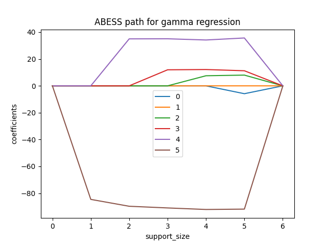
More on the Results

We can also plot the path of coefficients in abess process.

coef = np.zeros((7, 6))
loss = np.zeros(7)
for s in range(7):
    model = GammaRegression(support_size=s)
    model.fit(data.x, data.y)
    coef[s, :] = model.coef_
    loss[s] = model.eval_loss_

for i in range(6):
    plt.plot(coef[:, i], label=i)

plt.xlabel('support_size')
plt.ylabel('coefficients')
plt.title('ABESS path for gamma regression')
plt.legend()
plt.show()

The abess R package also supports Poisson regression and Gamma regression. For R tutorial, please view https://abess-team.github.io/abess/articles/v04-PoissonGammaReg.html.