Work with geomstats

The package geomstats is used for computations and statistics on nonlinear manifolds, such as Hypersphere,Hyperbolic Space, Symmetric-Positive-Definite (SPD) Matrices Space and Skew-Symmetric Matrices Space. abess also works well with the package geomstats. Here is an example of using abess to do logistic regression of samples on Hypersphere, and we will compare the precision score, the recall score and the running time with abess and with scikit-learn.

import numpy as np
import matplotlib.pyplot as plt
import geomstats.backend as gs
import geomstats.visualization as visualization
from geomstats.learning.frechet_mean import FrechetMean
from geomstats.geometry.hypersphere import Hypersphere
from sklearn.model_selection import train_test_split
from sklearn.metrics import precision_score, recall_score
from sklearn.linear_model import LogisticRegression as sklLogisticRegression
from abess import LogisticRegression
import time
import warnings
warnings.filterwarnings("ignore")
gs.random.seed(0)

INFO: Using numpy backend

An Example

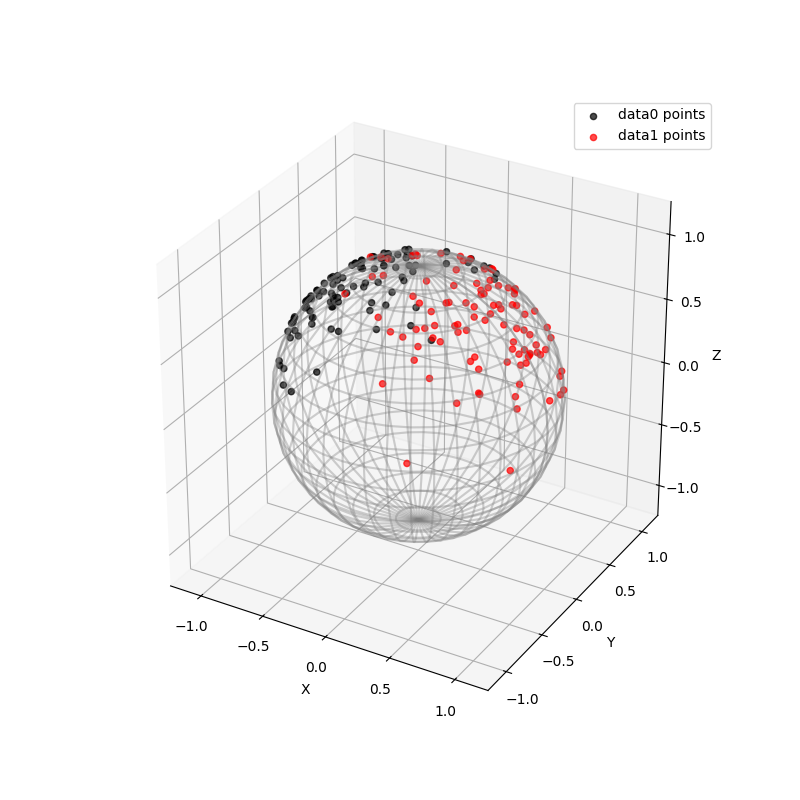
Two sets of samples on Hypersphere in 3-dimensional Euclidean Space are created. The sample points in data0 are distributed around \([-3/5, 0, 4/5]\), and the sample points in data1 are distributed around \([3/5, 0, 4/5]\). The sample size of both is set to 100, and the precision of both is set to 5. The two sets of samples are shown in the figure below.

sphere = Hypersphere(dim=2)
data0 = sphere.random_riemannian_normal(mean=np.array([-3/5, 0, 4/5]), n_samples=100, precision=5)
data1 = sphere.random_riemannian_normal(mean=np.array([3/5, 0, 4/5]), n_samples=100, precision=5)

fig = plt.figure(figsize=(8, 8))
ax = visualization.plot(data0, space="S2", color="black", alpha=0.7, label="data0 points")
ax = visualization.plot(data1, space="S2", color="red", alpha=0.7, label="data1 points")
ax.set_box_aspect([1, 1, 1])
ax.legend()
plt.show()

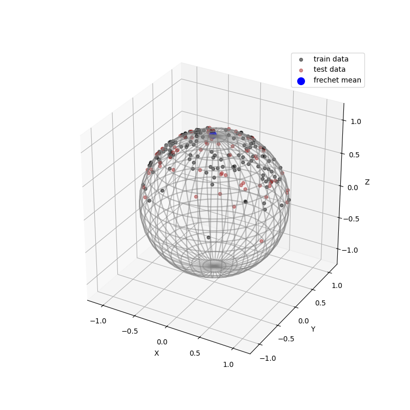
Then, we divide the data into train_data and test_data, and calculate the frechit mean of train_data, which has the minimum sum of the squares of the distances along the geodesic to each sample point in train_data. The test_data,the train_data and the frechit mean are shown in the figure below.

labels = np.concatenate((np.zeros(data0.shape[0]),np.ones(data1.shape[0])))
data = np.concatenate((data0,data1))
train_data, test_data, train_labels, test_labels = train_test_split(data, labels, test_size=0.33, random_state=0)

mean = FrechetMean(sphere)
mean.fit(train_data)
mean_estimate = mean.estimate_

fig = plt.figure(figsize=(8, 8))
ax = visualization.plot(train_data, space="S2", color="black", alpha=0.5, label="train data")
ax = visualization.plot(test_data, space="S2", color="brown", alpha=0.5, label="test data")
ax = visualization.plot(mean_estimate, space="S2", color="blue", s=100, label="frechet mean")
ax.set_box_aspect([1, 1, 1])
ax.legend()
plt.show()

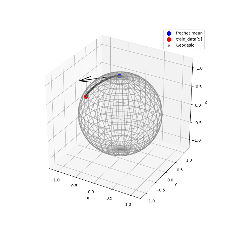
Next, do the logarithm map for all sample points from the frechit mean. That is, map each sample point to which point on the tangential of the geodesic (from the frechit mean to the sample point) at the frechit mean and has the distance to the frechit that equals to the length of the geodesic.

log_train_data = sphere.metric.log(train_data, mean_estimate)
log_test_data = sphere.metric.log(test_data, mean_estimate)

The following figure shows the logarithm mapping of train_data[5] from the frechit mean.

geodesic = sphere.metric.geodesic(mean_estimate, end_point=train_data[5])
points_on_geodesic = geodesic(gs.linspace(0.0, 1.0, 30))

fig = plt.figure(figsize=(8, 8))
ax = fig.add_subplot(111, projection="3d")
ax = visualization.plot(mean_estimate, space="S2", color="blue", s=100, label="frechet mean")
ax = visualization.plot(train_data[5], space="S2", color="red", s=100, label="train_data[5]")
ax = visualization.plot(points_on_geodesic, ax=ax, space="S2", color="black", alpha=0.5, label="Geodesic")
arrow = visualization.Arrow3D(mean_estimate, vector=log_train_data[5])
arrow.draw(ax, color="black")
ax.legend();
plt.show()

After that, the samples are naturally distributed on a linear area. Then, some common analysis methods can be used to analyze this set of data, such as LogisticRegression from abess.

model = LogisticRegression(support_size= range(0,4))
model.fit(log_train_data, train_labels)
fitted_labels = model.predict(log_test_data)

print('Used variables\' index:', np.nonzero(model.coef_ != 0)[0])
print('accuracy:',sum((fitted_labels - test_labels + 1) % 2)/test_data.shape[0])

Used variables' index: [0]
accuracy: 0.9090909090909091

The result shows that the only variables' index it used is \([0]\). When constructing the samples, the means of the two sets are only different in the 0th direction. It shows that abess correctly identifies the most relevant variable for classification.

Comparison

Here is the comparison of the precision score and the recall score with abess and scikit-learn, and the comparison of the running time with abess and scikit-learn.

We loop 50 times. At each time, two sets of samples on Hypersphere in 10-dimensional Euclidean Space are created. The sample points in data0 are distributed around \([1 / 3, 0, 2 / 3, 0, 2 / 3, 0, 0, 0, 0, 0]\), and the sample points in data1 are distributed around \([0, 0, 2 / 3, 0, 2 / 3, 0, 0, 0, 0, 1 / 3]\). The sample size of both is set to 200, and the precision of both is set to 5.

m = 50  # cycles
n_sam = 200
s = 10
pre = 5

sphere = Hypersphere(dim=s - 1)
labels = np.concatenate((np.zeros(n_sam), np.ones(n_sam)))
abess_precision_score = np.zeros(m)
skl_precision_score = np.zeros(m)
abess_recall_score = np.zeros(m)
skl_recall_score = np.zeros(m)
abess_geo_time = np.zeros(m)
skl_geo_time = np.zeros(m)

for i in range(m):
    data0 = sphere.random_riemannian_normal(mean=np.array([1 / 3, 0, 2 / 3, 0, 2 / 3, 0, 0, 0, 0, 0]), n_samples=n_sam,
                                            precision=pre)
    data1 = sphere.random_riemannian_normal(mean=np.array([0, 0, 2 / 3, 0, 2 / 3, 0, 0, 0, 0, 1 / 3]), n_samples=n_sam,
                                            precision=pre)
    data = np.concatenate((data0, data1))
    train_data, test_data, train_labels, test_labels = train_test_split(data, labels, test_size=0.33, random_state=0)
    mean = FrechetMean(sphere)
    mean.fit(train_data)
    mean_estimate = mean.estimate_
    log_train_data = sphere.metric.log(train_data, mean_estimate)
    log_test_data = sphere.metric.log(test_data, mean_estimate)

    start = time.time()
    abess_geo_model = LogisticRegression(support_size=range(0, s + 1)).fit(log_train_data, train_labels)
    abess_geo_fitted_labels = abess_geo_model.predict(log_test_data)
    end = time.time()
    abess_geo_time[i] = end - start
    abess_precision_score[i] = precision_score(test_labels, abess_geo_fitted_labels, average='micro')
    abess_recall_score[i] = recall_score(test_labels, abess_geo_fitted_labels, average='micro')

    start = time.time()
    skl_geo_model = sklLogisticRegression().fit(X=log_train_data, y=train_labels)
    skl_geo_fitted_labels = skl_geo_model.predict(log_test_data)
    end = time.time()
    skl_geo_time[i] = end - start
    skl_precision_score[i] = precision_score(test_labels, skl_geo_fitted_labels, average='micro')
    skl_recall_score[i] = recall_score(test_labels, skl_geo_fitted_labels, average='micro')

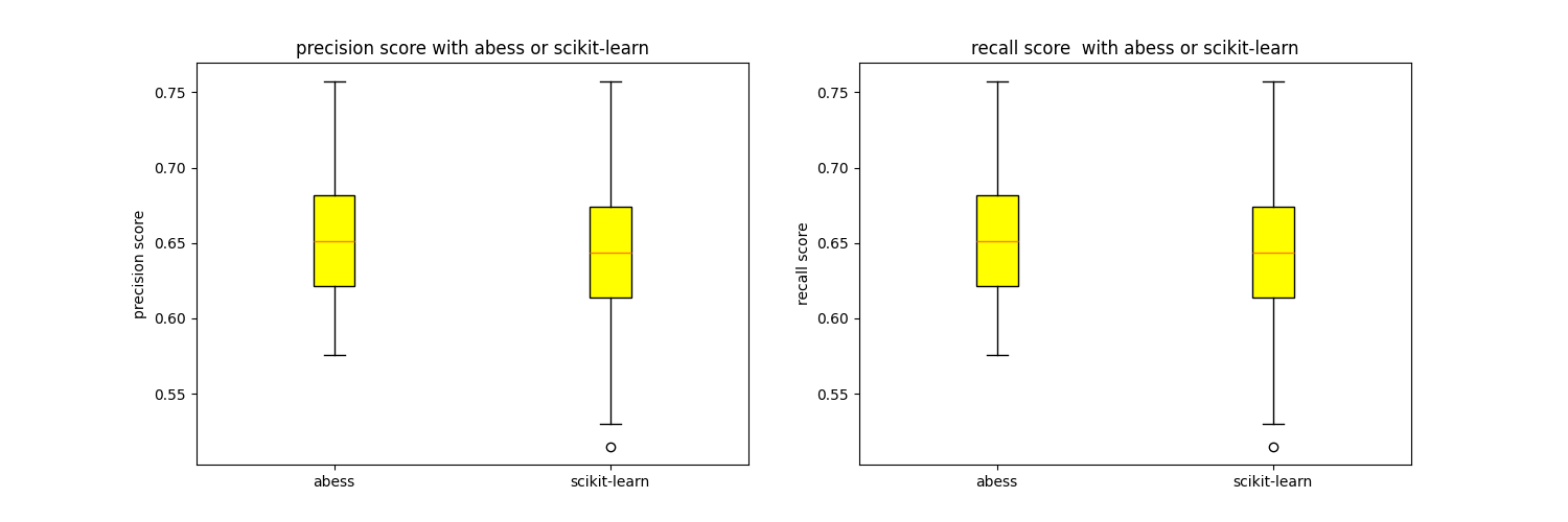
The following figures show the precision score and the recall score with abess or scikit-learn.

fig = plt.figure(figsize=(15,5))
ax1 = fig.add_subplot(121)
ax1.boxplot([abess_precision_score, skl_precision_score],
           patch_artist='Patch',
           labels = ['abess', 'scikit-learn'],
           boxprops = {'color':'black','facecolor':'yellow'}

          )
ax1.set_title('precision score with abess or scikit-learn')
ax1.set_ylabel('precision score')

ax2 = fig.add_subplot(122)
ax2.boxplot([abess_recall_score, skl_recall_score],
           patch_artist='Patch',
           labels = ['abess', 'scikit-learn'],
           boxprops = {'color':'black','facecolor':'yellow'}

          )
ax2.set_title('recall score  with abess or scikit-learn')
ax2.set_ylabel('recall score')
plt.show()

The following figure shows the running time with abess or scikit-learn.

abess_geo_time_mean = np.mean(abess_geo_time)
skl_geo_time_mean = np.mean(skl_geo_time)
abess_geo_time_std = np.std(abess_geo_time)
skl_geo_time_std = np.std(skl_geo_time)
meth = ['abess', 'scikit-learn']
x_pos = np.arange(len(meth))
CTEs = [abess_geo_time_mean, skl_geo_time_mean]
error = [abess_geo_time_std, skl_geo_time_std]

fig = plt.figure(figsize=(8,5))
ax = fig.add_subplot(111)
ax.bar(x_pos, CTEs, yerr=error, align='center', alpha=0.5, ecolor='black', capsize=10)
ax.set_ylabel('running time')
ax.set_xticks(x_pos)
ax.set_xticklabels(meth)
ax.set_title('running time with abess or scikit-learn')
ax.yaxis.grid(True)
plt.show()

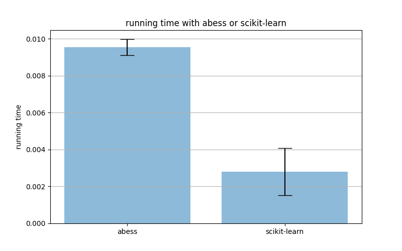
We can find that the precision score and the recall score with abess are generally higher than those without abess. And the running time with abess is only slightly slower than that without abess.

sphinx_gallery_thumbnail_path = 'Tutorial/figure/geomstats.png'