Specific Models

Introduction

From the algorithm preseneted in “ABESS algorithm: details”, one of the bottleneck in algorithm is the computation of forward and backward sacrifices, which requires conducting iterative algorithms or frequently visiting \(p\) variables. To improve computational efficiency, we designed specialize strategies for computing forward and backward sacrifices for different models. The specialize strategies is roughly divide into two classes: (i) covariance update for (multivariate) linear model; (ii) quasi Newton iteration for non-linear model (e.g., logistic regression). We going to specify the two strategies as follows.

Covariance update

Under linear model, the core bottleneck is computing sacrifices, e.g. the foreward sacrifices,

\[\zeta_{j}=\mathcal{L}_{n}\left(\hat{\boldsymbol{\beta}^{\mathcal{A}}}\right)-\mathcal{L}_{n}\left(\hat{\boldsymbol{\beta}}^{\mathcal{A}}+\hat{t}^{\{j\}}\right)=\frac{X_{j}^{\top} X_{j}}{2 n}\left(\frac{\hat{\boldsymbol d}_{j}}{X_{j}^{\top} X_{j} / n}\right)^{2}.\]

where \(\hat{t}=\arg \min _{t} \mathcal{L}_{n}\left(\hat{\boldsymbol{\beta}}^{\mathcal{A}}+t^{\{j\}}\right), \hat{\boldsymbol d}_{j}=X_{j}^{\top}(y-X \hat{\boldsymbol{\beta}}) / n\). Intuitively, for \(j \in \mathcal{A}\) (or \(j \in \mathcal{I}\) ), a large \(\xi_{j}\) (or \(\zeta_{j}\)) implies the \(j\) th variable is potentially important.

It would take a lot of time on calculating \(X^T_jy\), \(X^T_jX_j\) and its inverse. To speed up, it is actually no need to recompute these items at each splicing process. Instead, they can be stored when first calculated, which is what we call "covariance update".

It is easy to enable this feature with an additional argument covariance_update=True for linear model, for example:

import numpy as np
from time import time
from abess.linear import LinearRegression
from abess.datasets import make_glm_data

np.random.seed(1)
data = make_glm_data(n=10000, p=100, k=10, family='gaussian')
model1 = LinearRegression()
model2 = LinearRegression(covariance_update=True)

t1 = time()
model1.fit(data.x, data.y)
t1 = time() - t1

t2 = time()
model2.fit(data.x, data.y)
t2 = time() - t2

print(f"No covariance update: {t1}")
print(f"Covariance update: {t2}")
print(f"Same answer? {(model1.coef_==model2.coef_).all()}")

No covariance update: 2.1501963138580322
Covariance update: 2.071284532546997
Same answer? True

We can see that covariance update improve computation when sample size \(n\) is much larger than dimension \(p\).

However, we have to point out that covariance update will cause higher memory usage, especially when \(p\) is large. So, we recommend to enable covariance update for fast computation when sample size is much larger than dimension and dimension is moderate (\(p \leq 2000\)).

Quasi Newton iteration

In the third step in Algorithm 2 , we need to solve a convex optimization problem:

\[\tilde{\beta} = \arg\min_{\text{supp}(\beta) = \tilde{\mathcal{A}} } l_n(\beta ).\]

But generally, it has no closed-form solution, and has to be solved via iterative algorithm. A natural method for solving this problem is Netwon method, i.e., conduct the update:

\[\beta_{\tilde{\mathcal{A}} }^{m+1} \leftarrow \boldsymbol \beta_{\tilde{\mathcal{A}} }^m - \Big( \left.\frac{\partial^2 l_n( \boldsymbol \beta )}{ (\partial \boldsymbol \beta_{\tilde{\mathcal{A}}} )^2 }\right|_{\boldsymbol \beta = \boldsymbol \beta^m} \Big)^{-1} \Big( \left.\frac{\partial l_n( \boldsymbol \beta )}{ \partial \boldsymbol \beta_{\tilde{\mathcal{A}}} }\right|_{\boldsymbol \beta = \boldsymbol \beta^m} \Big),\]

until \(\| \beta_{\tilde{\mathcal{A}} }^{m+1} - \beta_{\tilde{\mathcal{A}} }^{m}\|_2 \leq \epsilon\) or \(m \geq k\), where \(\epsilon, k\) are two user-specific parameters. Generally, setting \(\epsilon = 10^{-6}\) and \(k = 80\) achieves desirable estimation. Generally, the inverse of second derivative is computationally intensive, and thus, we approximate it with its diagonalized version. Then, the update formulate changes to:

\[\beta_{\tilde{\mathcal{A}} }^{m+1} \leftarrow \boldsymbol \beta_{\tilde{\mathcal{A}} }^m - \rho D \Big( \left.\frac{\partial l_n( \boldsymbol \beta )}{ \partial \boldsymbol \beta_{\tilde{\mathcal{A}}} }\right|_{\boldsymbol \beta = \boldsymbol \beta^m} \Big),\]

where \(D = \textup{diag}( (\left.\frac{\partial^2 l_n( \boldsymbol \beta )}{ (\partial \boldsymbol \beta_{\tilde{\mathcal{A}_{1}}} )^2 }\right|_{\boldsymbol \beta = \boldsymbol \beta^m} )^{-1}, \ldots, (\left.\frac{\partial^2 l_n( \boldsymbol \beta )}{ (\partial \boldsymbol \beta_{\tilde{\mathcal{A}}_{|A|}} )^2 }\right|_{\boldsymbol \beta = \boldsymbol \beta^m} )^{-1})\) and \(\rho\) is step size. Although using the approximation may increase the iteration time, it avoids a large computational complexity when computing the matrix inversion. Furthermore, we use a heuristic strategy to reduce the iteration time. Observing that not every new support after exchanging the elements in active set and inactive set may not reduce the loss function, we can early stop the newton iteration on these support. Specifically, support \(l_1 = L({\beta}^{m}), l_2 = L({\beta}^{m+1})\), if \(l_1 - (k - m - 1) \times (l_2 - l_1)) > L - \tau\), then we can expect the new support cannot lead to a better loss after \(k\) iteration, and hence, it is no need to conduct the remaining \(k - m - 1\) times Newton update. 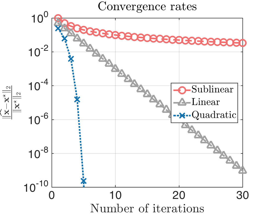This heuristic strategy is motivated by the convergence rate of Netwon method is linear at least.

To enable this feature, you can simply give an additional argument approximate_Newton=True. The \(\epsilon\) and \(k\) we mentioned before, can be set with primary_model_fit_epsilon and primary_model_fit_max_iter, respectively. For example:

import numpy as np
from time import time
from abess.linear import LogisticRegression
from abess.datasets import make_glm_data

np.random.seed(1)
data = make_glm_data(n=1000, p=100, k=10, family='binomial')
model1 = LogisticRegression()
model2 = LogisticRegression(approximate_Newton=True,
                            primary_model_fit_epsilon=1e-6,
                            primary_model_fit_max_iter=10)

t1 = time()
model1.fit(data.x, data.y)
t1 = time() - t1

t2 = time()
model2.fit(data.x, data.y)
t2 = time() - t2

print(f"No newton: {t1}")
print(f"Newton: {t2}")
print(f"Same answer? {(np.nonzero(model1.coef_)[0]==np.nonzero(model2.coef_)[0]).all()}")

No newton: 6.584152460098267
Newton: 2.3175113201141357
Same answer? True

The abess R package also supports covariance update and quasi Newton iteration. For R tutorial, please view https://abess-team.github.io/abess/articles/v09-fasterSetting.html