Work with pyts

pyts is a Python package dedicated to time series classification. It aims to make time series classification easily accessible by providing preprocessing and utility tools, and implementations of several time series classification algorithms. In this example, we will mainly focus on the shapelets-based algorithms.

Shapelets learning is a new primitive in time series classification. Shapelets are defined as subsequences of time series that are in some sense maximally representative of a class. Informally, in a binary classification task, a shapelet is discriminant if it is present in most series of one class and absent from series of the other class. ShapeletTransform is a powerful method implemented by pyts to perform shapelets-based feature transformation. Actually, abess also works well with shapelets-based methods. This example shows how to effectively select discriminant shapelets with abess.

import numpy as np
import matplotlib.pyplot as plt
import time
import warnings
warnings.filterwarnings('ignore')
from abess.linear import LogisticRegression
from sklearn.svm import LinearSVC
from sklearn.pipeline import make_pipeline
from pyts.transformation import ShapeletTransform
from pyts.datasets import load_coffee

Data

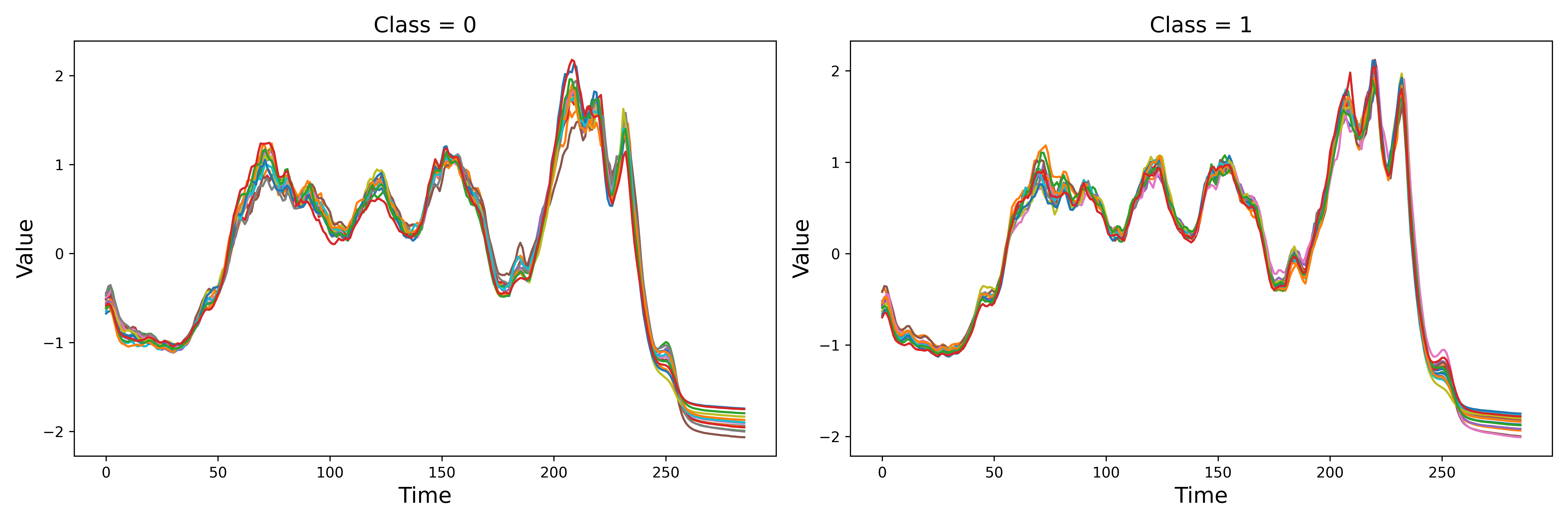
In this example, we use the buint-in coffee dataset in pyts to perform shapelets learning. It has two classes, 0 and 1. So, this is a binary classification task. Both train dataset and test dataset have 28 time series and the dimension of each time series is 286. We plot the time series in the train dataset.

X_train, X_test, y_train, y_test = load_coffee(return_X_y=True)
print("X_train shape: ", X_train.shape)
print("X_test shape: ", X_test.shape)

fig, (ax1, ax2) = plt.subplots(1, 2, figsize=(15, 5), dpi=600)
ax1.plot(X_train[y_train == 0].T)
ax1.set_title("Class = 0", fontsize=15)
ax1.set_xlabel("Time", fontsize=15)
ax1.set_ylabel("Value", fontsize=15)
ax2.plot(X_train[y_train == 1].T)
ax2.set_title("Class = 1", fontsize=15)
ax2.set_xlabel("Time", fontsize=15)
ax2.set_ylabel("Value", fontsize=15)
fig.tight_layout()
plt.show()

X_train shape:  (28, 286)
X_test shape:  (28, 286)

Learning shapelets with abess

To select discriminant shapelets, we first collect all subsequences with predefined length and step as the candidates. Then we transform the original time series by computing the distance between them to each subsequence. Therefore, the original time series are transformed to some ultra high dimensional vectors. Finally, we perform binary classification and shapelets selection simultaneously with LogisticRegression implemented by abess.

class abessShapelet(object):

    def __init__(self, X_train, X_test, y_train, y_test, len_shapelet=None, step=None):
        self.X_train = X_train
        self.X_test = X_test
        self.y_train = y_train
        self.y_test = y_test
        self.n, self.p = X_train.shape
        if len_shapelet == None:
            len_shapelet = int(self.p / 4)
        if step == None:
            step = int(len_shapelet / 2)
        num_each = 1 + (self.p - len_shapelet) // step
        self.shapelets = []
        for i in range(self.n):
            for j in range(num_each):
                col = j*step
                self.shapelets.append(self.X_train[i, col:(col+len_shapelet)])
        self.shapelets = np.array(self.shapelets)

    def distant(self, x, y):
        assert x.ndim == 1 and y.ndim == 1
        n_x = len(x)
        n_y = len(y)
        if n_x <= n_y:
            dist = np.zeros(n_y-n_x+1)
            for i in range(n_y-n_x+1):
                shapelet = y[i:i+n_x]
                dist[i] = np.sum((x-shapelet)**2)
            return dist.min()
        else:
            dist = np.zeros(n_x-n_y+1)
            for i in range(n_x-n_y+1):
                shapelet = x[i:i+n_y]
                dist[i] = np.sum((y-shapelet)**2)
            return dist.min()

    def featureTransform(self, X, shapelets, index=None):
        if index is None:
            index = np.arange(shapelets.shape[0])
        n, p = X.shape
        num_shapelets, k = shapelets.shape
        new_feature = np.zeros((n, num_shapelets))
        for i in range(n):
            for j in index:
                new_feature[i, j] = self.distant(X[i], shapelets[j])
        return new_feature

    def fit_predict(self, size=None):
        X_train_new = self.featureTransform(self.X_train, self.shapelets)
        model = LogisticRegression(support_size=size)
        model.fit(X_train_new, self.y_train)
        self.index = np.nonzero(model.coef_)[0]
        X_test_new = self.featureTransform(
            self.X_test, self.shapelets, self.index)
        y_pred = model.predict(X_test_new)
        return y_pred

In the following, we perform shapelets learning using abessShapelet. We print the performance and execution time.

t1 = time.time()
aShapelet = abessShapelet(X_train, X_test, y_train, y_test, len_shapelet=75)
y_pred = aShapelet.fit_predict(size=2)
score_abess = (y_pred == y_test).mean()
t2 = time.time()
print("score_abess: ", round(score_abess, 2))
print("time_abess : {}s".format(round(t2 - t1, 2)))

score_abess:  0.96
time_abess : 6.13s

Learning shapelets with pyts

We compare our method with the one implemented in pyts, which is a two-step procedure. First, it selects discriminant shapelets based on mutual information. Then, a support vector machine is applied to perform binary classification with transformed time series based on those selected shapelets. Analogously, we print the performance and execution time.

t3 = time.time()
shapelet = ShapeletTransform(n_shapelets=2, window_sizes=[75], sort=True)
svc = LinearSVC()
clf = make_pipeline(shapelet, svc)
clf.fit(X_train, y_train)
score_pyts = clf.score(X_test, y_test)
t4 = time.time()
print("score_pyts: ", round(score_pyts, 2))
print("time_pyts : {}s".format(round(t4 - t3, 2)))

score_pyts:  0.96
time_pyts : 24.76s

It can be seen from the above results that the linear classifier abessShapelet obtains the same performance with the method implemented by pyts while the running time is much shorter.

Plot: learned shapelets

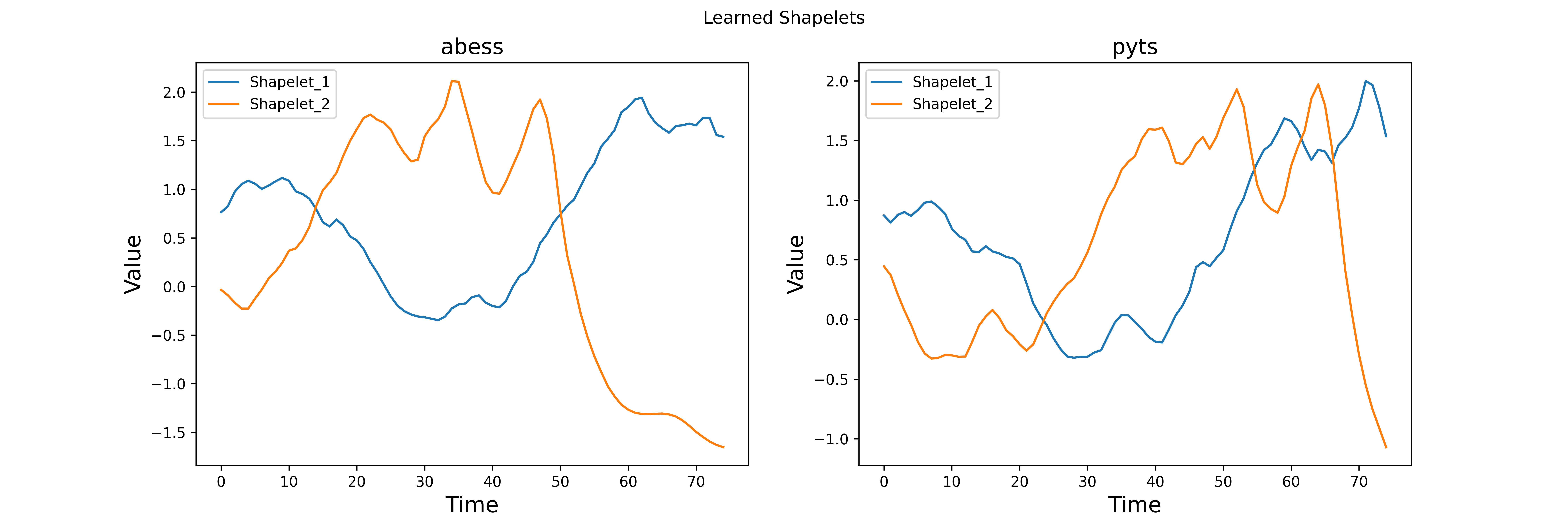
The following figure shows the discriminant shapelets selected by these two methods.

fig, (ax1, ax2) = plt.subplots(1, 2, figsize=(15, 5), dpi=600)

ax1.plot(aShapelet.shapelets[aShapelet.index][0], label="Shapelet_1")
ax1.plot(aShapelet.shapelets[aShapelet.index][1], label="Shapelet_2")
ax1.legend()
ax1.set_title("abess", fontsize=15)
ax1.set_xlabel("Time", fontsize=15)
ax1.set_ylabel("Value", fontsize=15)

ax2.plot(shapelet.shapelets_[0], label="Shapelet_1")
ax2.plot(shapelet.shapelets_[1], label="Shapelet_2")
ax2.legend()
ax2.set_title("pyts", fontsize=15)
ax2.set_xlabel("Time", fontsize=15)
ax2.set_ylabel("Value", fontsize=15)

plt.suptitle("Learned Shapelets")
plt.show()

sphinx_gallery_thumbnail_path = 'Tutorial/figure/pyts.png'