Note
Go to the end to download the full example code.
Work with DoWhy#
DoWhy is a Python library for causal inference that supports explicit modeling and testing of causal assumptions. In
this section, we will use abess to cope with high-dimensional mediation analysis problem, which is a popular topic in
the research of causal inference. High-Dimensional mediation model is crucial in biomedical research studies. People always
want to know by what mechanism the genes with differential expression, distinct genotypes or various epigeneticmarkers affect
the outcome or phenotype. Such a mechanistic process is what a mediation analysis aims to characterize (Huang and Pan, 2016 2 ).
A typical example of the high-dimensional mediators is high-dimensional DNA methylation markers. This model can be represented by the following figure (Zhang et al. 2016 1 ),
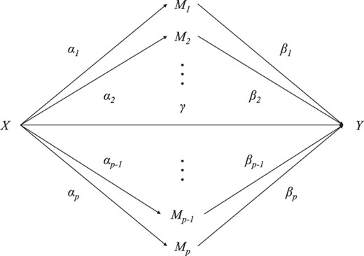
where \(X\) is treatment (exposure), \(Y\) is outcome, and \(M_k,k=1,...,p\) are (potential) mediators. Moreover,
\(\alpha=\left(\alpha_{1}, \cdots, \alpha_{p}\right)^{\mathrm{T}}\) denotes the parameters relating \(X\) to mediators,
and \(\beta=\left(\beta_{1}, \cdots, \beta_{p}\right)^{\mathrm{T}}\) denotes the parameters relating the mediators to
the outcome \(Y\). For the latter relation, we would consider both continuous outcomes (linear regression) and
binary outcomes (logistic regression). These two models can be implemented by abess directly.
For instance, if the outcome is continuous, then we assume the model take the form
Among all the possible \(M_p\) (\(p\) may be large), only few of them are real mediators, which means that both \(\alpha_k\) and \(\beta_k\) should be non-zero. Then, an indirect path \(X \rightarrow M_k \rightarrow Y\) can be built. Next, we will show that by directly using ABESS in a naive form, we can get a good result.
Continuous Outcome#
We will follow the simulation settings and the data generating process in the R document of the R package HIMA (Zhang et al. 2016). \(X\) is generated from \(N(0,1.5)\), the first 8 elements of \(\beta\left(\beta_{k}, k=1, \cdots, 8\right)\) are \((0.55,0.6,0.65,0.7,0.8,0.8,0,0)^{\mathrm{T}}\), and the first 8 elements of \(a\left(\alpha_{k}, k=1, \cdots, 8\right)\) are \((0.45,0.5,0.6,0.7,0,0,0.5,0.5)^{\mathrm{T}}\). The rest of \(\beta\) and \(\alpha\) are all 0 . Let \(c=1, \gamma=0.5. c_{k}\) is chosen as a random number from \(U(0,2) . e_{k}\) and \(\epsilon\) are generated from \(N(0,1.2)\) and \(N(0,1)\), respectively.
import numpy as np
import pandas as pd
import random
import abess
import math
from dowhy import CausalModel
import dowhy.datasets
import dowhy.causal_estimators.linear_regression_estimator
import warnings
warnings.filterwarnings('ignore')

# The data-generating function:

def simhima (n,p,alpha,beta,seed,binary=False):
    random.seed(seed)
    ck = np.random.uniform(0,2,size=p)
    M = np.zeros((n,p))
    X = np.random.normal(0,1.5,size=n)
    for i in range(n):
        e = np.random.normal(0,1.2,size=p)
        M[i,:] = ck + X[i]*alpha + e
    X = X.reshape(n,1)
    XM = np.concatenate((X,M),axis=1)
    B = np.concatenate((np.array([0.5]),beta),axis=0)
    E = np.random.normal(0,1,size=n)
    Y = 0.5 + np.matmul(XM,B) + E
    if binary:
        Y = np.random.binomial(1,1/(1+np.exp(Y)),size=n)
    return {"Y":Y, "M":M, "X":X}

n = 300
p = 200
alpha = np.zeros(p)
beta = np.zeros(p)
alpha[0:8] = (0.45,0.5,0.6,0.7,0,0,0.5,0.5)
beta[0:8] = (0.55,0.6,0.65,0.7,0.8,0.8,0,0)
simdat = simhima(n,p,alpha,beta,seed=12345)
Now, let's examine again our settings. There are altogether \(p=200\) possible mediators, but only few of them are the true mediators that we really want to find out. A true mediator must have both non-zero \(\alpha\) and \(\beta\), so only the first four mediators satisfy this condition (indices 0,1,2,3). We also set up four false mediators that are easily confused (indices 4,5,6,7), which have either non-zero \(\alpha\) or \(\beta\), and should avoid being selected by our method.
The whole structure can be divided into left and right parts. The left part is about the paths \(X \rightarrow M_i, i=1,2,...p\),
and the right part is about the paths \(M_i \rightarrow Y, i=1,2,...p\). A natural idea is to apply abess to these two subproblems
separately. Notice: the right part is in the same form as the problem abess wants to solve: one dependent variable and multiple
possible independent variables, but the left part is opposite: we have one independent variable and multiple possible dependent
variables. In this case, continuing to naively use abess may lead to philosophical causal issues and cannot have good theoretical
guarantees, since we have to treat \(X\) as an "dependent variable" and treat \(M_i\) as "independent variables", which is contrary
to the interpretation in reality. However, this naive approach performs well in this task of selecting true mediators, and this
kind of idea has already been used in some existing methods, such as Coordinate-wise Mediation Filter (Van Kesteren and Oberski, 2019 3 ).
Therefore, we will still use this kind of idea here, and the main task is to show the power of abess.
We will first apply BESS with a fixed support size to one of these subproblems, conducting a preliminary screening to determine some candidate mediators, and then apply ABESS with an adaptive size to the second subproblem and decide the final selected mediators. If we directly use ABESS in the first subproblem, the candidate set would be too small, and make the ABESS in the second step meaningless (because the candidate set is no longer high-dimensional at this time), which could induce a large drop of TPR (True Positive Rate). The support size used in the first step can be tuned, and its size is preferably 2 to 4 times the number of true mediators.
Now there is a problem of order. Since we have to run abess twice, should we do the left half or the right half first?
We've found that doing the left half first is almost always a better choice. The reason is as follows: if we do the right
half first, those false mediators that only have correlation coefficients with the left half will be easily selected because
there is an \(M_i \leftarrow X \rightarrow Y\) path (note that from \(X\) to \(Y\) has not only indirect paths, but also a direct path!),
and once these false mediators are selected into the second step, they will be selected eventually because they have non-zero
coefficients in the left half, resulting in uncontrollable FDR. But doing the left half first won't have such a problem.
model = abess.LinearRegression(support_size=10)
model.fit(simdat["M"],simdat["X"])
ind = np.nonzero(model.coef_)
print("estimated non-zero: ", ind)
print("estimated coef: ", model.coef_[ind])
estimated non-zero:  (array([  0,   1,   2,   3,   6,   7,  46, 112, 124, 185]),)
estimated coef:  [ 0.19938462  0.14855243  0.27148782  0.23536246  0.15900585  0.23215292
 -0.10422092 -0.11303449  0.09631314 -0.08907528]
This the subproblem of left half, and we use a "support size=10" to demonstrate conveniently. These 10 mediators have been selected in the first step and entered our candidate set for the second step. Recall that the true mediators we want to find have index 0,1,2,3. They are all selected in the candidate set.
model1 = abess.LinearRegression()
model1.fit(simdat["M"].T[ind].T,simdat["Y"])
ind1 = np.nonzero(model1.coef_)
print("estimated non-zero: ", ind[0][ind1])
recorded_index = ind[0][ind1]
estimated non-zero: [0 1 2 3 7]
This is the second step, and we use an adaptive support size, which lead to a final selection: index 0,1,2,3. We've
perfectly accomplished the task of selecting real mediators. After this step, we can use the DoWhy library for
our data for further analysis.
m_num = len(recorded_index)
df = pd.DataFrame(simdat["M"].T[recorded_index].T, columns=["FD"+str(i) for i in range(m_num)])
df["y"] = simdat["Y"]
df["v0"] = simdat["X"]
df.head()
In order to adapt to the naming convention of the DoWhy library, we renamed the above variables. v0 is treatment,
y is outcome, and FD0 to FD3 (short for Front Door) are mediators.
data = dowhy.datasets.linear_dataset(0.5, num_common_causes=0, num_samples=300,
                                     num_instruments=0, num_effect_modifiers=0,
                                     num_treatments=1,
                                     num_frontdoor_variables=m_num,
                                     treatment_is_binary=False,
                                    outcome_is_binary=False)
my_graph = data["gml_graph"][:-1] + ' edge[ source "v0" target "y"]]'
model = CausalModel(df,"v0","y",my_graph,
                   missing_nodes_as_confounders=True)
model.view_model()
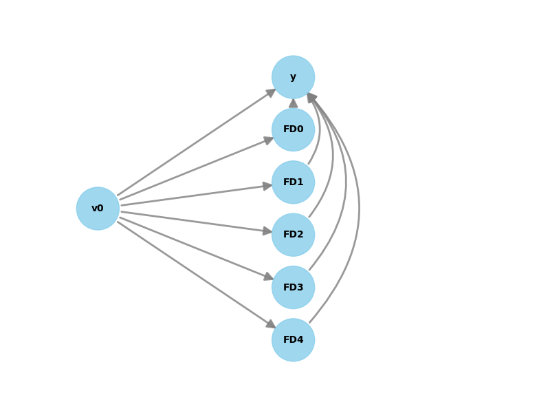
DoWhy library can directly display the causal graph we built. Now we can do identification and estimation based
on this causal graph and the data we simulated with DoWhy. For example, we are going to estimate the
natural indirect effect (NIE) of the first mediator \(M_0\) (FD0).
identified_estimand_nie = model.identify_effect(estimand_type="nonparametric-nie",
                                            proceed_when_unidentifiable=True)
causal_estimate_nie = model.estimate_effect(identified_estimand_nie,
                                        method_name="mediation.two_stage_regression",
                                       confidence_intervals=False,
                                       test_significance=False,
                                        method_params = {
                                            'first_stage_model': dowhy.causal_estimators.linear_regression_estimator.LinearRegressionEstimator,
                                            'second_stage_model': dowhy.causal_estimators.linear_regression_estimator.LinearRegressionEstimator
                                        }
                                       )
print("The estimate of the natural indirect effect of the first mediator is ",causal_estimate_nie.value)
The estimate of the natural indirect effect of the first mediator is 0.3381542041456464
Recall that we have \(\alpha_0=0.45\) and \(\beta_0=0.55\), the true value of the natural indirect effect of the first mediator is \(0.45 \times 0.55 = 0.2475\). Similarly, we can also get the estimated value of NIE of other mediator variables, and also the natural direct effect (NDE). Since the linear regression model has a simple and known form in our simulation, it's obvious that the accuracy of our estimates depends only on whether we choose the correct mediators. Next, we would do 1000 replications and see the performance of abess on choosing mediators.
recorded_index = ind[0][ind1]
for i in range(999):
    simdat = simhima(n,p,alpha,beta,seed=i)
    model = abess.LinearRegression(support_size=10)
    model.fit(simdat["M"],simdat["X"])
    ind = np.nonzero(model.coef_)
    model1 = abess.LinearRegression()
    model1.fit(simdat["M"].T[ind].T,simdat["Y"])
    ind1 = np.nonzero(model1.coef_)
    recorded_index = np.concatenate((recorded_index,ind[0][ind1]),axis=0)
mask = np.unique(recorded_index)
tmp = []
for v in mask:
    tmp.append(np.sum(recorded_index==v))
np.vstack((mask,np.array(tmp))).T
array([[   0,  985],
       [   1,  998],
       [   2, 1000],
       [   3, 1000],
       [   4,   21],
       [   5,   20],
       [   6,   40],
       [   7,   39],
       [  31,    1],
       [  46,    1],
       [  54,    1],
       [  57,    1],
       [  73,    1],
       [  81,    1],
       [  83,    1],
       [  84,    1],
       [  91,    1],
       [ 102,    1],
       [ 128,    1],
       [ 147,    1],
       [ 159,    1],
       [ 168,    1],
       [ 175,    1],
       [ 177,    1]])
After doing 1000 replications of the process mentioned above, we can get this list. The left number in each row is the index, and the right number is the times that this mediator been selected. We can find that:
The true mediators (indices 0-3) can always be selected during all the 1000 replications.
The bewildering false mediators (indices 4-7) may be occasionally selected, but FDR can be controlled at a low level.
It is almost impossible for other mediators (indices 8-199) to be selected by our method.
Now, we can do the confusion matrix analysis, and output some commonly used metrics to measure our selection method.
Positive = 4*1000
Negative = 196*1000
TP = np.sum(tmp[:4])
FP = np.sum(tmp[4:])
FN = Positive-TP
TN = Negative-FP
TPR = TP/Positive
TNR = TN/Negative
PPV = TP/(TP+FP)
FDR = 1-PPV
ACC = (TP+TN)/(Positive+Negative)
F1 = 2*TP/(2*TP+FP+FN)
print('TPR:',TPR,'\nTNR:',TNR,'\nFDR:',FDR,'\nPPV:',PPV,'\nACC:',ACC,'\nF1 score:',F1)
TPR: 0.99575
TNR: 0.9993061224489795
FDR: 0.033017722748239886
PPV: 0.9669822772517601
ACC: 0.999235
F1 score: 0.9811553146939278
Binary Outcome#
For binary outcome, we still follow the simulation settings of the R documentation of the R package HIMA. We increased the sample size from 300 to 600, which is also a reasonable size.
First step:
model = abess.LinearRegression(support_size=10)
model.fit(simdat["M"],simdat["X"])
ind = np.nonzero(model.coef_)
print("estimated non-zero: ", ind)
print("estimated coef: ", model.coef_[ind])
estimated non-zero:  (array([  0,   1,   2,   3,   6,   7,  52, 154, 168, 197]),)
estimated coef:  [ 0.22098081  0.18630423  0.2115897   0.3276324   0.14303822  0.22073874
 -0.06781737 -0.06798672 -0.06352619  0.05718398]
Second step:
model1 = abess.LogisticRegression()
model1.fit(simdat["M"].T[ind].T,simdat["Y"])
ind1 = np.nonzero(model1.coef_)
print("estimated non-zero: ", ind[0][ind1])
recorded_index = ind[0][ind1]
estimated non-zero: [0 1 2 3]
Again, we got a perfect result.
recorded_index = ind[0][ind1]
for i in range(999):
    simdat = simhima(n,p,alpha,beta,seed=i,binary=True)
    model = abess.LinearRegression(support_size=10)
    model.fit(simdat["M"],simdat["X"])
    ind = np.nonzero(model.coef_)
    model1 = abess.LogisticRegression()
    model1.fit(simdat["M"].T[ind].T,simdat["Y"])
    ind1 = np.nonzero(model1.coef_)
    recorded_index = np.concatenate((recorded_index,ind[0][ind1]),axis=0)
mask = np.unique(recorded_index)
tmp = []
for v in mask:
    tmp.append(np.sum(recorded_index==v))
np.vstack((mask,np.array(tmp))).T
array([[  0, 903],
       [  1, 934],
       [  2, 959],
       [  3, 986],
       [  4,  25],
       [  5,  21],
       [  6,   2],
       [  7,   7],
       [ 37,   1],
       [111,   1],
       [136,   1],
       [143,   1],
       [146,   1],
       [188,   2]])
TPR has dropped significantly because problems with binary outcomes require a larger sample size than problems with continuous outcomes. But we found that FDR was also well controlled.
Positive = 4*1000
Negative = 196*1000
TP = np.sum(tmp[:4])
FP = np.sum(tmp[4:])
FN = Positive-TP
TN = Negative-FP
TPR = TP/Positive
TNR = TN/Negative
PPV = TP/(TP+FP)
FDR = 1-PPV
ACC = (TP+TN)/(Positive+Negative)
F1 = 2*TP/(2*TP+FP+FN)
print('TPR:',TPR,'\nTNR:',TNR,'\nFDR:',FDR,'\nPPV:',PPV,'\nACC:',ACC,'\nF1 score:',F1)
TPR: 0.9455
TNR: 0.9996836734693878
FDR: 0.016129032258064502
PPV: 0.9838709677419355
ACC: 0.9986
F1 score: 0.9643039265680775
In a word, by simply using abess in high-dimensional mediation analysis problem, we can get good results both
under continuous and binary outcome settings.
References
- 1
Zhang H, Zheng Y, Zhang Z, Gao T, Joyce B, Yoon G, Zhang W, Schwartz J, Just A, Colicino E, Vokonas P, Zhao L, Lv J, Baccarelli A, Hou L & Liu L (2016). “Estimating and Testing High-dimensional Mediation Effects in Epigenetic Studies.” Bioinformatics, 32(20), 3150-3154. (doi.org/10.1093/bioinformatics/btw351).
- 2
Huang YT & Pan WC (2016). “Hypothesis test of mediation effect in causal mediation model with high‐dimensional continuous mediators.” Biometrics, 72(2), 402-413. (doi.org/10.1111/biom.12421)
- 3
Van Kesteren, E. J., & Oberski, D. L. (2019). “Exploratory mediation analysis with many potential mediators.” Structural Equation Modeling: A Multidisciplinary Journal, 26(5), 710-723. (doi.org/10.1080/10705511.2019.1588124)
sphinx_gallery_thumbnail_path = 'Tutorial/figure/dowhy.png'
Total running time of the script: (0 minutes 42.776 seconds)