Work with DoubleML

Double machine learning 1 offer a debiased way for estimating low-dimensional parameter of interest in the presence of high-dimensional nuisance. Many machine learning methods can be used to estimate the nuisance parameters, such as random forests, lasso or post-lasso, neural nets, boosted regression trees, and so on. The Python package DoubleML 2 provide an implementation of the double machine learning. It's built on top of scikit-learn and is an excellent package. The object-oriented implementation of DoubleML is very flexible, in particular functionalities to estimate double machine learning models and to perform statistical inference via the methods fit, bootstrap, confint, p_adjust and tune.

In fact, abess 3 also works well with the package DoubleML. Here is an example of using abess to solve such a problem, and we will compare it to the lasso regression.

import numpy as np
from sklearn.base import clone
from sklearn.linear_model import LassoCV
from abess.linear import LinearRegression
from doubleml import DoubleMLPLR
import matplotlib.pyplot as plt
import warnings             # ignore warnings
warnings.filterwarnings('ignore')
import time

Partially linear regression (PLR) model

PLR models take the form

\[\begin{split}Y=D \theta_{0}+g_{0}(X)+U, & \quad\mathbb{E}(U \mid X, D)=0,\\ D=m_{0}(X)+V, & \quad\mathbb{E}(V \mid X)=0,\end{split}\]

where \(Y\) is the outcome variable, \(D\) is the policy/treatment variable. \(\theta_0\) is the main regression coefficient that we would like to infer, which has the interpretation of the treatment effect parameter. The high-dimensional vector \(X=(X_1,\dots, X_p)\) consists of other confounding covariates, and \(U\) and \(V\) are stochastic errors. Usually, \(p\) is not vanishingly small relative to the sample size, it's difficult to estimate the nuisance parameters \(\eta_0 = (m_0, g_0)\). abess aims to solve general best subset selection problem. In PLR models, abess is applicable when nuisance parameters are sparse. Here, we are going to use abess to estimate the nuisance parameters, then combine with DoubleML to estimate the treatment effect parameter.

Data

We simulate the data from a PLR model, which both \(m_0\) and \(g_0\) are low-dimensional linear combinations of \(X\), and we save the data as DoubleMLData class.

from doubleml import DoubleMLData
np.random.seed(1234)
n_obs = 200
n_vars = 600
theta = 3
X = np.random.normal(size=(n_obs, n_vars))
d = np.dot(X[:, :3], np.array([5]*3)) + np.random.standard_normal(size=(n_obs,))
y = theta * d + np.dot(X[:, :3], np.array([5]*3)) + np.random.standard_normal(size=(n_obs,))
dml_data_sim = DoubleMLData.from_arrays(X, y, d)

Model fitting with abess

Based on the simulated data, now we are going to illustrate how to integrate the abess with DoubleML. To estimate the PLR model with the double machine learning algorithm, first we need to choose a learner to estimate the nuisance parameters \(\eta_0 = (m_0, g_0)\). Considering the sparsity of the data, we can use the adaptive best subset selection model. Then fitting the model to learn the average treatment effct parameter \(\theta_0\).

abess = LinearRegression(cv = 5)      # abess learner
ml_g_abess = clone(abess)
ml_m_abess = clone(abess)

obj_dml_plr_abess = DoubleMLPLR(dml_data_sim, ml_g_abess, ml_m_abess)   # model fitting
obj_dml_plr_abess.fit();
print("thetahat:", obj_dml_plr_abess.coef)
print("sd:", obj_dml_plr_abess.se)

thetahat: [3.03421218]
sd: [0.07167669]

The estimated value is close to the true parameter, and the standard error is very small. abess integrates with DoubleML easily, and works well for estimating the nuisance parameter.

Comparison with lasso

The lasso regression is a shrinkage and variable selection method for regression models, which can also be used in high-dimensional setting. Here, we compare the abess regression with the lasso regression at different variable dimensions.

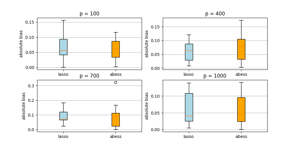
The following figures show the absolute bias of the abess learner and the lasso learner.

lasso = LassoCV(cv = 5)     # lasso learner
ml_g_lasso = clone(lasso)
ml_m_lasso = clone(lasso)

M = 15      # repeate times
n_obs = 200
n_vars_range = range(100,1100,300)    # different dimensions of confounding covariates
theta_lasso = np.zeros(len(n_vars_range)*M)
theta_abess = np.zeros(len(n_vars_range)*M)
time_lasso = np.zeros(len(n_vars_range)*M)
time_abess = np.zeros(len(n_vars_range)*M)
j = 0

for n_vars in n_vars_range:
    for i in range(M):
        np.random.seed(i)
        # simulated data: three true variables
        X = np.random.normal(size=(n_obs, n_vars))
        d = np.dot(X[:, :3], np.array([5]*3)) + np.random.standard_normal(size=(n_obs,))
        y = theta * d + np.dot(X[:, :3], np.array([5]*3)) + np.random.standard_normal(size=(n_obs,))
        dml_data_sim = DoubleMLData.from_arrays(X, y, d)

        # Estimate double/debiased machine learning models
        starttime = time.time()
        obj_dml_plr_lasso = DoubleMLPLR(dml_data_sim, ml_g_lasso, ml_m_lasso)
        obj_dml_plr_lasso.fit()
        endtime = time.time()
        time_lasso[j*M + i] = endtime - starttime
        theta_lasso[j*M + i] = obj_dml_plr_lasso.coef

        starttime = time.time()
        obj_dml_plr_abess = DoubleMLPLR(dml_data_sim, ml_g_abess, ml_m_abess)
        obj_dml_plr_abess.fit()
        endtime = time.time()
        time_abess[j*M + i] = endtime - starttime
        theta_abess[j*M + i] = obj_dml_plr_abess.coef
    j = j + 1

# absolute bias
abs_bias1 = [abs(theta_lasso-theta)[:M],abs(theta_abess-theta)[:M]]
abs_bias2 = [abs(theta_lasso-theta)[M:2*M],abs(theta_abess-theta)[M:2*M]]
abs_bias3 = [abs(theta_lasso-theta)[2*M:3*M],abs(theta_abess-theta)[2*M:3*M]]
abs_bias4 = [abs(theta_lasso-theta)[3*M:4*M],abs(theta_abess-theta)[3*M:4*M]]
labels = ["lasso", "abess"]

fig, ([ax1, ax2], [ax3, ax4]) = plt.subplots(nrows=2, ncols=2, figsize=(10,5))
bplot1 = ax1.boxplot(abs_bias1, vert=True, patch_artist=True, labels=labels)
ax1.set_title("p = 100")
bplot2 = ax2.boxplot(abs_bias2, vert=True, patch_artist=True, labels=labels)
ax2.set_title("p = 400")
bplot3 = ax3.boxplot(abs_bias3, vert=True, patch_artist=True, labels=labels)
ax3.set_title("p = 700")
bplot4 = ax4.boxplot(abs_bias4, vert=True, patch_artist=True, labels=labels)
ax4.set_title("p = 1000")
colors = ["lightblue", "orange"]

for bplot in (bplot1, bplot2, bplot3, bplot4):
    for patch, color in zip(bplot["boxes"], colors):
        patch.set_facecolor(color)
for ax in [ax1, ax2, ax3, ax4]:
    ax.yaxis.grid(True)
    ax.set_ylabel("absolute bias")
plt.show();

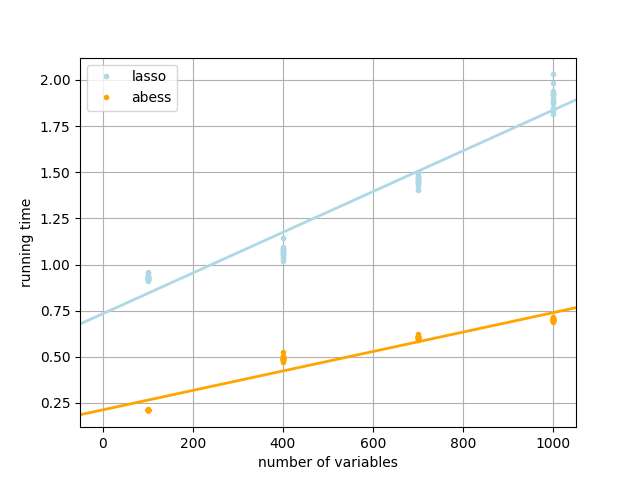
The following figure shows the running time of the abess learner and the lasso learner.

plt.plot(np.repeat(n_vars_range, M),time_lasso, "o", color = "lightblue", label="lasso", markersize=3);
plt.plot(np.repeat(n_vars_range, M),time_abess, "o", color = "orange", label="abess", markersize=3);
slope_lasso, intercept_lasso = np.polyfit(np.repeat(n_vars_range, M),time_lasso, 1)
slope_abess, intercept_abess = np.polyfit(np.repeat(n_vars_range, M),time_abess, 1)
plt.axline(xy1=(0,intercept_lasso), slope = slope_lasso, color = "lightblue", lw = 2)
plt.axline(xy1=(0,intercept_abess), slope = slope_abess, color = "orange", lw = 2)
plt.grid()
plt.xlabel("number of variables")
plt.ylabel("running time")
plt.legend(loc="upper left")

<matplotlib.legend.Legend object at 0x7f951ca95f10>

At each dimension, we repeat the double machine learning procedure 15 times for each of the two learners. As can be seen from the above figures, the parameters estimated by both learners are very close to the true parameter \(\theta_0\). But the running time of abess learner is much shorter than lasso. Besides, in high-dimensional situations, the mean absolute bias of abess learner regression is relatively smaller.

References

1

Chernozhukov V, Chetverikov D, Demirer M, et al. Double/debiased machine learning for treatment and structural parameters[M]. Oxford University Press Oxford, UK, 2018.

2

Bach P, Chernozhukov V, Kurz M S, et al. Doubleml-an object-oriented implementation of double machine learning in python[J]. Journal of Machine Learning Research, 2022, 23(53): 1-6.

3

Zhu J, Hu L, Huang J, et al. abess: A fast best subset selection library in python and r[J]. arXiv preprint arXiv:2110.09697, 2021.

sphinx_gallery_thumbnail_path = 'Tutorial/figure/doubleml.png'